Download
1 / 28
490 likes | 1.09k Views
Continuous Time Convolution . In this animation, the continuous time convolution of signals is discussed. Convolution is the operation to obtain response of a linear system to input x(t). The output y(t) is given as a weighted superposition of impulse responses, time shifted by .

E N D
Continuous Time Convolution In this animation, the continuous time convolution of signals is discussed. Convolution is the operation to obtain response of a linear system to input x(t). The output y(t) is given as a weighted superposition of impulse responses, time shifted by Course Name: Signals and Systems Level: UG Author Phani Swathi Chitta Mentor Prof. Saravanan Vijayakumaran
Learning Objectives After interacting with this Learning Object, the learner will be able to: • Explain the convolution of two continuous time signals
Definitions of the components/Keywords: 1 Convolution of two signals: Let x(t) and h(t) are two continuous signals to be convolved. The convolution of two signals is denoted by which means where t is the variable of integration. 2 3 4 5
f(t) g(t) 2 2 1 ** t t --22 22 1 Master Layout 1 Signals taken to convolve 2 3 Output of the convolution y(t) 1 4 t -2 0 2 3 5
f(t) = 2 g(t)= -t+1 2 2 1 t t --22 22 1 Step 1: 1 2 3 4 5
g(t-t) 2 2 g(-t) f(t) f(t) 1 1 t t -1 + t -2 -2 2 2 Step 2: 1 2 -1 t Fig. a Fig. b 3 4 5
g(t-t) 2 f(t) 1 t -1 + t -2 2 Step 3: Calculation of y(t) in five stages 1 Stage - I : t < -2 2 t 3 4 5
2 g(t-t) f(t) 1 t -1 + t -2 2 Step 4: 1 Stage - II : -2 ≤ t < -1 2 t 3 4 5
2 g(t-t) f(t) 1 t -2 -1 + t 2 Step 5: 1 Stage - III : -1 ≤ t < 2 2 t 3 4 5
f(t) 2 g(t-t) 1 t -2 -1 + t Step 6: 1 Stage - IV : 2 ≤ t < 3 2 2 t 3 4 5
f(t) 2 g(t-t) 1 t -2 2 -1 + t Step 7: 1 Stage - V : t ≥ 3 2 t 3 4 5
Step 8: Output of Convolution 1 y(t) 1 2 t 3 -2 0 2 3 4 5
Electrical Engineering Slide 1 Slide 3 Slide 24-26 Slide 28 Slide 27 Introduction Definitions Analogy Test your understanding (questionnaire) Lets Sum up (summary) Want to know more… (Further Reading) f(t ) and g(t-t ) Interactivity: Try it yourself +1 g(t) f(t) +1 +1 t -1 t t -1 -1 f(t ) g(t-t ) Select Select +1 +1 +1 t -1 -1 +1 +1 t -1 13 The four signals must be repeated under select for both f(t) and g(t) Credits
Electrical Engineering Slide 1 Slide 3 Slide 24-26 Slide 28 Slide 27 Introduction Definitions Analogy Test your understanding (questionnaire) Lets Sum up (summary) Want to know more… (Further Reading) f(t ) and g(t-t ) Interactivity: Try it yourself +1 g(t) f(t) +1 +1 t -1 t t -1 -1 f(t ) g(t-t ) Select Select +1 +1 +1 t -1 -1 +1 +1 t -1 14 The signal selected under f(t) must be shown Credits
Electrical Engineering Slide 1 Slide 3 Slide 24-26 Slide 28 Slide 27 Introduction Definitions Analogy Test your understanding (questionnaire) Lets Sum up (summary) Want to know more… (Further Reading) f(t ) and g(t-t ) Interactivity: Try it yourself +1 g(t) f(t) +1 +1 t -1 t t -1 -1 f(t ) g(t-t ) Select Select +1 +1 +1 t -1 -1 +1 +1 t -1 15 The signal selected under g(t) must be shown Credits
Electrical Engineering Slide 1 Slide 3 Slide 24-26 Slide 28 Slide 27 Introduction Definitions Analogy Test your understanding (questionnaire) Lets Sum up (summary) Want to know more… (Further Reading) f(t ) and g(t-t ) Interactivity: +1 Try it yourself g(t) f(t) +1 +1 t -1 t t -1 -1 f(t ) g(t-t ) Select Select +1 +1 +1 t -1 -1 +1 +1 t -1 16 The red figure is the shifted and reversed version of g(t) The slides 16-21 should be shown in a smooth fashion Credits
Electrical Engineering Slide 1 Slide 3 Slide 24-26 Slide 28 Slide 27 Introduction Definitions Analogy Test your understanding (questionnaire) Lets Sum up (summary) Want to know more… (Further Reading) f(t ) and g(t-t ) Interactivity: Try it yourself +1 g(t) f(t) +1 +1 t -1 t t -1 -1 f(t ) g(t-t ) Select Select +1 +1 +1 t -1 -1 +1 +1 t -1 17 Credits
Electrical Engineering Slide 1 Slide 3 Slide 24-26 Slide 28 Slide 27 Introduction Definitions Analogy Test your understanding (questionnaire) Lets Sum up (summary) Want to know more… (Further Reading) f(t ) and g(t-t ) Interactivity: Try it yourself +1 g(t) f(t) +1 +1 t -1 t t -1 -1 f(t ) g(t-t ) Select Select +1 +1 +1 t -1 -1 +1 +1 t -1 18 Credits
Electrical Engineering Slide 1 Slide 3 Slide 24-26 Slide 28 Slide 27 Introduction Definitions Analogy Test your understanding (questionnaire) Lets Sum up (summary) Want to know more… (Further Reading) f(t ) and g(t-t ) Interactivity: Try it yourself +1 g(t) f(t) +1 +1 t -1 t t -1 -1 f(t ) g(t-t ) Select Select +1 +1 +1 t -1 -1 +1 +1 t -1 19 Credits
Electrical Engineering Slide 1 Slide 3 Slide 24-26 Slide 28 Slide 27 Introduction Definitions Analogy Test your understanding (questionnaire) Lets Sum up (summary) Want to know more… (Further Reading) f(t ) and g(t-t ) Interactivity: Try it yourself +1 g(t) f(t) +1 +1 t -1 t t -1 -1 f(t ) g(t-t ) Select Select +1 +1 +1 t -1 -1 +1 +1 t -1 20 Credits
Electrical Engineering Slide 1 Slide 3 Slide 24-26 Slide 28 Slide 27 Introduction Definitions Analogy Test your understanding (questionnaire) Lets Sum up (summary) Want to know more… (Further Reading) f(t ) and g(t-t ) Interactivity: Try it yourself +1 g(t) f(t) +1 +1 t -1 t t -1 -1 f(t ) g(t-t ) Select Select +1 +1 +1 t -1 -1 +1 +1 t -1 21 Credits
Electrical Engineering Slide 1 Slide 3 Slide 24-26 Slide 28 Slide 27 Introduction Definitions Analogy Test your understanding (questionnaire) Lets Sum up (summary) Want to know more… (Further Reading) f(t) +1 +1 +1 * t -1 -1 -1 f(t) +1 +1 * t -1 +1 +1 +1 * -1 -1 -1 22 The same procedure is done to the above given combination of signals Credits
Electrical Engineering Slide 1 Slide 3 Slide 24-26 Slide 28 Slide 27 Introduction Definitions Analogy Test your understanding (questionnaire) Lets Sum up (summary) Want to know more… (Further Reading) +1 +1 * -1 +1 +1 * 23 The same procedure is done to the above given combination of signals Credits
Questionnaire 1 1. If the unit-impulse response of an LTI system and the input signal both are rectangular pulses, then the output will be a Answers: a) rectangular pulse b) triangular pulse c) ramp function d) none of the above 2. Find Convolution * Answers: a) b) 2 x(t) δ(t-5) 3 5 4 5 5 5
Questionnaire 1 3. If impulse response and input signal both are unit step responses, then the output will be * Answers: a) Triangular pulse b) Unit step function c) Ramp function d) None of the above 4. The convolution integral is given by i) ii) Hint: let Answers: a) i b) ii c) Both i and ii d)either i or ii 2 3 4 5
Questionnaire 1 5. If h(t) is a unit-step function and x(t) is a unit-ramp function, then the output y(t) will be a Answers: a) step function b) ramp function c) Triangular pulse d) Quadratic function 2 3 4 5
Links for further reading Reference websites: Books: Signals & Systems – Alan V. Oppenheim, Alan S. Willsky, S. Hamid Nawab, PHI learning, Second edition. Signals and Systems – Simon Haykin, Barry Van Veen, John Wiley & Sons, Inc. Research papers:
Summary • The convolution operation is used to obtain the output of linear time – invariant system in response to an arbitrary input. • In continuous time, the representation of signals is taken to be the weighted integrals of shifted unit impulses. • The convolution integral of two continuous signals is represented as where • The convolution integral provides a concise, mathematical way to express the output of an LTI system based on an arbitrary continuous-time input signal and the system‘s response.