Download
1 / 22
220 likes | 348 Views
PIC Simulation of Fast Ignition Targets with OSIRIS. J. Tonge, M. Tzoufras, J. Fahlen, B. J. Winjum, F. S. Tsung, W. B. Mori, UCLA C. Ren, Rochester M. Marti, R. Fonseca, L. O. Silva, IST. How much laser energy can we get into the Core?.

E N D
PIC Simulation of Fast Ignition Targets with OSIRIS J. Tonge, M. Tzoufras, J. Fahlen, B. J. Winjum, F. S. Tsung, W. B. Mori, UCLA C. Ren, Rochester M. Marti, R. Fonseca, L. O. Silva, IST
How much laser energy can we get into the Core? • What are the characteristics, energy spectrum and spread, of the fast electrons generated by the laser plasma interaction? • How are fast electrons be transported through plasma to the Core? • How do the fast electrons interact with the Core? • How do these effect each other?
Code Development and Scientific Discovery in Parallel • Scientific Discovery is incremental • New code developments yields new scientific results • New scientific results guide code development priorities
Overview • Recent Code Improvements • Simulation Results • Absorbing core • Target density profile • Future Code improvements
Simulation Technology • Load balancing: • Static real 4x speed up of simulations vs no load balancing. • Reduced numeric heating: • Quadratic spline current deposition and field interpolation scheme + current smoothing. • Core: • Add particle drag to core. This adds current termination at core. Not an attempt at first principles implementation.
Improved Energy Conservation Allows lower temperature and higher density Dx/lD=10.6 (100 nc 1.3 kev) Quadratic Spline + 3 pass Smoother Dx/lD=6.7 (40nc 1.3 kev) Quadratic Spline + 4,1 pass Smoother Dx/lD=2.8 (40 nc 7.6 kev) Quadratic Spline + 4,1 pass Smoother Dx/lD=2.8 (40nc 7.6 kev) Area Weighting + 4,1 pass Smoother
Resistive Core Target • Target radius 51 mm diameter • Linear slope to max density (100 nc) at 16 mm • Resistive Core • 6.4mm diameter • Drag ( g-1) on electrons within core. • No drag on particles with Energy less than ~12Te or greater than 10MeV. 100nc 16m 3m 25.5m laser 100m
Compressed Target Data Courtesy R. Betti, Rochester
PIC Simulation Target and Setup • Isolated target with vacuum region between target and boundary • Resistive Core. • Peak Target Density(nt) = 100nc • 1256012560 grids • xmax=0.5 c/p • quadratic spline & current smoothing • 2.6 108 particles and 7.4104 steps • 71 hours on 128 cpu’s (on Dawson) • Initial Te= 1.3 keV, Ti=1 keV • 1m Laser • I=1020-21 w/cm2 • spot size (FWHM) 7.5 m (scaled) • 1 ps long, p-polarized.
Core Heating • 1 kJ Laser • 4% efficiency • 40 Joules into core with 3.2 mm radius • Core Density ~ 1026 cm-3 • Would heat core to 12 kev
Shallow Density Gradient Target • Vacuum region between target and boundary • Target core Density(nt) = 100nc • Surrounding plasma with linear density gradient • 1203212032 grids • (x=0.5 c/p ) • quadratic spline & current smoothing • 2.4 108 particles and 6104 steps • Initial Te=1.3 keV, Ti=1 keV • 1-laser, • I=1020-21 w/cm2 • spot size (FWHM) 7.5 • 1 ps long, p-polarized
Interaction Region 397 fsLaser and current filamention B field n = 100 nc Te = 1.3 keV Shallow gradient target 4.5 nc/m n = 100 nc Te = 1.3 keV Steep gradient target 10.5 nc/m
Interaction Region 397 fsLaser and current filamention B field n = 100 nc Te = 1.3 keV n = 40 nc Te = 7.4 keV n = 40 nc Te = 1.3 keV n= 40 nc targets have 4.2 nc/m density gradient n= 100 nc target has 10.5 nc/m density gradient
Simulation Technology • Load balancing: • dynamic - may provide additional 1.5x to 2x speed improvement. • Boundary conditions: • Better isolation of boundaries using perfectly matched (PML) boundary conditions (Vay). • Core: • Add position dependent 2-particle collisions. (Takizuka, Nanbu)
Collisions (IST) Collision of same species • Sort particle buffer by collision cells • Calculate particle statistics for each collision cell • Pair the particles randomly • For each pair: • calculate the number of collisions within the current collision cycle • calculate a sample of the deflection angle • deflect the momentum of the collision partners according to this deflection angle. This corresponds to a rotation of the respective momentum in the center of mass reference frame of the pair Even number Odd number Pic Cell Collision Cell Same number Different number Collision of different species
Summary • Improved current deposition scheme, core and load balancing. • Simulations show a few percent of Laser power is deposited in core. • Filament size and length changes in Laser particle interaction region due to change in target profile. • New simulation technology: Improved Boundary conditions, Load balancing, Collisional core.