Download
1 / 40
530 likes | 852 Views
Graph Theory. Chapter 6 . In the beginning…. 1736: Leonhard Euler Basel, 1707-St. Petersburg, 1786 He wrote A solution to a problem concerning the geometry of a place. First paper in graph theory. Problem of the Königsberg bridges:

E N D
Graph Theory Chapter 6
In the beginning… • 1736: Leonhard Euler • Basel, 1707-St. Petersburg, 1786 • He wrote A solution to a problem concerning the geometry of a place. First paper in graph theory. • Problem of the Königsberg bridges: • Starting and ending at the same point, is it possible to cross all seven bridges just once and return to the starting point?
Some important names • Thomas Pennington Kirkman (Manchester, England 1806-1895) • British clergyman who studied combinatorics. • William Rowan Hamilton (Dublin, Ireland 1805-1865) • applied "quaternions" • worked on optics, dynamics and analysis • created the "icosian game" in 1857, a precursor of Hamiltonian cycles. • Denes Konig (Budapest, Hungary 1844-1944) • Interested in four-color problem and graph theory • 1936: publishes Theory of finite and infinite graphs, thefirst textbook on graph theory
What is a graph G? It is a pair G = (V, E), where V = V(G) = set of vertices E = E(G) = set of edges Example: V = {s, u, v, w, x, y, z} E = {(x,s), (x,v)1, (x,v)2, (x,u), (v,w), (s,v), (s,u), (s,w), (s,y), (w,y), (u,y), (u,z),(y,z)} 6.1 Introduction
Edges • An edge may be labeled by a pair of vertices, for instance e = (v,w). • e is said to be incident on v and w. • Isolated vertex = a vertex without incident edges.
Special edges • Parallel edges • Two or more edges joining a pair of vertices • in the example, a and b are joined by two parallel edges • Loops • An edge that starts and ends at the same vertex • In the example, vertex d has a loop
Simple graph A graph without loops or parallel edges. Weighted graph A graph where each edge is assigned a numerical label or “weight”. Special graphs
Directed graphs (digraphs) G is a directed graph or digraph if each edge has been associated with an ordered pair of vertices, i.e. each edge has a direction
Similarity graphs (1) Problem: grouping objects into similarity classes based on various properties of the objects. • Example: • Computer programs that implement the same algorithm have properties k = 1, 2 or 3 such as: • 1. Number of lines in the program • 2. Number of “return” statements • 3. Number of function calls
Similarity graphs (2) Suppose five programs are compared and a table is made:
Similarity graphs (3) • A graph G is constructed as follows: • V(G) is the set of programs {v1, v2, v3, v 4, v5 }. • Each vertex vi is assigned a triple (p1, p2, p3), • where pk is the value of property k = 1, 2, or 3 • v1 = (66,20,1) • v2 = (41, 10, 2) • v3 = (68, 5, 8) • v4 = (90, 34, 5) • v5 = (75, 12, 14)
Dissimilarity functions (1) • Define a dissimilarity function as follows: • For each pair of vertices v = (p1, p2, p3) and w = (q1, q2, q3) let 3 s(v,w) = |pk – qk| k = 1 • s(v,w) is a measure of dissimilarity between any two programs v and w • Fix a number N. Insert an edge between v and w if s(v,w) < N. Then: • We say that v and w are in the same class if v = w or if there is a path between v and w.
Dissimilarity functions (2) • Let N = 25. • s(v1,v3) = 24, s(v3,v5) = 20 and all other s(vi,vj) > 25 • There are three classes: • {v1,v3, v5}, {v2} and {v4} • The similarity graph looks like the picture
Complete graph K n • Let n > 3 • The complete graph Kn is the graph with n vertices and every pair of vertices is joined by an edge. • The figure represents K5
Bipartite graphs • A bipartite graph G is a graph such that • V(G) = V(G1) V(G2) • |V(G1)| = m, |V(G2)| = n • V(G1) V(G2) = • No edges exist between any two vertices in the same subset V(Gk), k = 1,2
Complete bipartite graph Km,n • A bipartite graph is the complete bipartite graph Km,n if every vertex in V(G1) is joined to a vertex in V(G2) and conversely, • |V(G1)| = m • |V(G2)| = n
Connected graphs • A graph is connected if every pair of vertices can be connected by a path • Each connected subgraph of a non-connected graph G is called a component of G
6.2 Paths and cycles • A path of length n is a sequence of n + 1 vertices and n consecutive edges • A cycle is a path that begins and ends at the same vertex
An Euler cycle in a graph G is a simple cycle that passes through every edge of G only once. The Königsberg bridge problem: Starting and ending at the same point, is it possible to cross all seven bridges just once and return to the starting point? This problem can be represented by a graph Edges represent bridges and each vertex represents a region. Euler cycles
Degree of a vertex • The degree of a vertex v, denoted by (v), is the number of edges incident on v • Example: • (a) = 4, (b) = 3, • (c) = 4, (d) = 6, • (e) = 4, (f) = 4, • (g) = 3.
Euler graphs • A graph G is an Euler graph if it has an Euler cycle. Theorems 6.2.17 and 6.2.18: G is an Euler graph if and only if G is connected and all its vertices have even degree. • The connected graph represents the Konigsberg bridge problem. • It is not an Euler graph. • Therefore, the Konigsberg bridge problem has no solution.
Sum of the degrees of a graph Theorem 6.2.21: If G is a graph with m edges and n vertices v1, v2,…, vn, then n (vi) = 2m i = 1 In particular, the sum of the degrees of all the vertices of a graph is even.
6.3 Hamiltonian cycles • Traveling salesperson problem • To visit every vertex of a graph G only once by a simple cycle. • Such a cycle is called a Hamiltonian cycle. • If a connected graph G has a Hamiltonian cycle, G is called a Hamiltonian graph.
Gray codes • Considered as a graph, a ring model for parallel computation is a cycle. • A Gray code is a sequence s1, s2,…, s2nsuch that • every n-bit string appears somewhere in the sequence • sk and sk+1 differ in exactly one bit • And s 2n and s1 differ in exactly one bit.
Parallel computation models (1) The n-cube In has 2n processors, n > 1 • Vertices are labeled 0, 1, 2,…, 2n-1 • An edge connects two vertices if the binary representation of their labels differs in exactly one bit • The n-cube simulates a ring model with 2n processors if it contains a simple cycle with 2n vertices which is a Hamiltonian cycle • The n-cube (n > 2) has a Gray code, therefore it contains a simple Hamiltonian cycle with 2n vertices, and so it is a model for parallel computation. • I1 has only two vertices 0 and 1. It has no cycles.
Parallel computation models (2) • I2 (a square) has 4 vertices labeled 00, 01, 10 and 11 • A Hamiltonian cycle is (00, 01, 11, 10, 00) • I3 (a cube) has 8 vertices labeled 000, 001, 010, 011, 100, 101 and 111 • A Hamiltonian cycle is (000, 001, 011, 010, 110, 111, 101, 100, 000)
The 3-cube The Hamiltonian cycle (000, 001, 011, 010, 110, 111, 101, 100, 000) joins vertices that differ by one bit.
I4 (the hypercube) has16 vertices, 32 edges and 20 faces Vertex labels: 0000 0001 0010 0011 0100 0101 0110 0111 1000 1001 1010 1011 1100 1101 1110 1111 The hypercube or 4-cube
6.4 A shortest-path algorithm • Due to Edsger W. Dijkstra, Dutch computer scientist born in 1930 • Dijkstra's algorithm finds the length of the shortest path from a single vertex to any other vertex in a connected weighted graph. • For a simple, connected, weighted graph with n vertices, Dijkstra’s algorithms has worst-case run time (n2).
6.5 Representations of graphs Adjacency matrix Rows and columns are labeled with ordered vertices write a 1 if there is an edge between the row vertex and the column vertex and 0 if no edge exists between them
Incidence matrix Label rows with vertices Label columns with edges 1 if an edge is incident to a vertex, 0 otherwise Incidence matrix
6.6 Isomorphic graphs G1 and G2 are isomorphic • if there exist one-to-one onto functions f: V(G1) → V(G2) and g: E(G1) → E(G2) such that • an edge e is adjacent to vertices v, w in G1 if and only if g(e) is adjacent to f(v) and f(w) in G2
6.7 Planar graphs A graph is planar if it can be drawn in the plane without crossing edges
Edges in series Edges in series: • If v V(G) has degree 2 and there are edges (v, v1), (v, v2) with v1 v2, • we say the edges (v, v1) and (v, v2) are in series.
A series reduction consists of deleting the vertex v V(G) and replacing the edges (v,v1) and (v,v2) by the edge (v1,v2) The new graph G’ has one vertex and one edge less than G and is said to be obtained from G by series reduction Series reduction
Homeomorphic graphs • Two graphs G and G’ are said to be homeomorphic if G’ is obtained from G by a sequence of series reductions. • By convention, G is said to be obtainable from itself by a series reduction, i.e. G is homeomorphic to itself. • Define a relation R on graphs: GRG’ if G and G’ are homeomorphic. • R is an equivalence relation on the set of all graphs.
Euler’s formula • If G is planar graph, • v = number of vertices • e = number of edges • f = number of faces, including the exterior face • Then: v – e + f = 2
Kuratowski’s theorem G is a planar graph if and only if G does not contain a subgraph homeomorphic to either K 5 or K 3,3
Isomorphism and adjacency matrices • Two graphs are isomorphic if and only if after reordering the vertices their adjacency matrices are the same