Download
1 / 18
200 likes | 465 Views
Graph Theory. Dijkstra. Single-Source Shortest Paths. We wish to find the shortest route between Binghamton and NYC. Given a NYS road map with all the possible routes how can we determine our shortest route?

E N D
Graph Theory Dijkstra
Single-Source Shortest Paths • We wish to find the shortest route between Binghamton and NYC. Given a NYS road map with all the possible routes how can we determine our shortest route? • We could try to enumerate all possible routes. It is certainly easy to see we do not need to consider a route that goes through Buffalo. Cutler/Head
Modeling Problem • We can model this problem with a directed graph. Intersections correspond to vertices, roads between intersections correspond to edges and distance corresponds to weights. One way roads correspond to the direction of the edge. • The problem: • Given a weighted digraph and a vertex s in the graph: find a shortest path from s to t Cutler/Head
1 8 s t A B -3 The distance of a shortest path Case 1: The graph may have negative edges but no negative cycles. The shortest distance from s to t can be computed. d(s,t)=6 • Case 2: The graph contains negative weight cycles, • and a path from s to t includes an edge on a negative • weight cycle. The shortest path distance is -. 1 8 1 d(s,t)=- s t A B -3 Cutler/Head
Shortest Path Algorithms • Dijkstra’s algorithm does NOT allow negative edges. • Uses a greedy heuristic. • undirected/directed graph • Bellman-Ford’s and Floyd’s algorithms work correctly for any graph and can detect negative cycles. • Must be directed graph if negative edges are included. Cutler/Head
Solving Optimization Problems • Often solved in 2 stages: • First Stage: solves an intermediate problem and saves an additional data structure. • Second Stage: uses the data Structure to construct the solution to the problem. Cutler/Head
Dijkstra’s shortest path algorithm Dijkstra’s algorithm solves the single source shortest path problem in 2 stages. • Stage1: A greedy algorithm computes the shortest distance from s to all other nodes in the graph and saves a data structure. • Stage2 : Uses the data structure for finding a shortest path from s to t. CS333 /Class 25
Main idea • Assume that the shortest distances from the starting node s to the rest of the nodes are d(s, s) d(s, s1) d(s, s2) … d(s, sn-1) • In this case a shortest path from s to si may include any of the vertices {s1, s2… si-1} but cannot include any sj where j > i. • Dijkstra’s main idea is to select the nodes and compute the shortest distances in the order s, s1, s2 ,…, sn-1 CS333 /Class 25
s4 8 15 s3 2 10 s s2 3 4 5 1 s1 • d(s, s) =0 • d(s, s1)=5 • d(s, s2)=6 • d(s, s3)=8 • d(s, s4)=15 Example Note: The shortest path from s to s2 includes s1 as an intermediate node but cannot include s3 or s4. Cutler/Head
Dijkstra’s greedy selection rule • Assume s1, s2… si-1 have been selected, and their shortest distances have been stored in Solution • Select node si and save d(s, si) if si has the shortest distance from s on a path that may include only s1, s2… si-1 as intermediate nodes. We call such paths special • To apply this selection rule efficiently, we need to maintain for each unselected node v the distance of the shortest special path from s to v, D[v]. Cutler/Head
s4 8 15 s3 2 10 s s2 3 4 5 1 s1 Solution = {(s, 0)} D[s1]=5 for path [s, s1] D[s2]= for path [s, s2] D[s3]=10 for path [s, s3] D[s4]=15 for path [s, s4]. Solution = {(s, 0), (s1, 5) } D[s2]= 6 for path [s, s1, s2] D[s3]=9 for path [s, s1, s3] D[s4]=15 for path [s, s4] Solution = {(s, 0), (s1, 5), (s2, 6) } D[s3]=8 for path [s, s1, s2, s3] D[s4]=15 for path [s, s4] Solution = {(s, 0), (s1, 5), (s2, 6),(s3, 8), (s4, 15) } Application Example Cutler/Head
s4 8 15 s3 2 10 s s2 3 4 5 1 s1 Implementing the selection rule • Node near is selected and added to Solution if D(near) D(v) for any v Ï Solution. Solution = {(s, 0)} D[s1]=5 D[s2]= D[s1]=5 D[s3]=10 D[s1]=5 D[s4]=15 Node s1 is selected Solution = {(s, 0), (s1, 5) } CS333 /Class 25
Updating D[ ] • After adding near to Solution, D[v] of all nodes v Ï Solution are updated if there is a shorter special path from s to v that contains node near, i.e., if (D[near] + w(near, v ) < D[v]) then D[v]=D[near] + w(near, v ) D[near ] = 5 2 Solution after adding near 2 3 s D[ v ] = 9 is updated to D[v]=5+2=7 3 6 CS333 /Class 25
s4 8 15 s3 2 10 s s2 3 4 5 1 s1 Updating D Example Solution = {(s, 0)} D[s1]=5, D[s2]= , D[s3]=10, D[s4]=15. Solution = {(s, 0), (s1, 5) } D[s2]= D[s1]+w(s1, s2)=5+1=6, D[s3]= D[s1]+w(s1, s3)=5+4=9, D[s4]=15 Solution = {(s, 0), (s1, 5), (s2, 6) } D[s3]=D[s2]+w(s2, s3)=6+2=8, D[s4]=15 Solution = {(s, 0), (s1, 5), (s2, 6), (s3, 8), (s4, 15) } Cutler/Head
Dijkstra’s Algorithm for Finding the Shortest Distance from a Single Source Dijkstra(G,s)1. for eachv V2. doD [ v ] 3. D [ s ] 04. PQ make-PQ(D,V)5. whilePQ 6. donear PQ.extractMin () 7. for eachv Adj(near )8 ifD [ v ] > D [ near ] +w( near ,v )9. then D [ v ] D [ near ] +w( near, v )10. PQ.decreasePriorityValue (D[v], v )11. return the label D[u] of each vertex u Cutler/Head
1. for eachv V2. doD [ v ] 3. D [ s ] 04. PQ make-PQ(D,V)5. whilePQ 6. donear PQ.extractMin () 7. for eachv Adj(near )8 ifD [ v ] > D [ near ] + w( near ,v )9. then D [ v ] D[near] + w(near,v)10. PQ.decreasePriorityValue (D[v ], v )11. return the label D[u] of each vertex u Assume a node in PQ can be accessed in O(1) ** Decrease key for v requires O(lgV ) provided the node in heap with v’s data can be accessed in O(1) Using Heap implementation Lines 1 -4 run in O (V ) Max Size of PQ is | V | (5) Loop = O (V ) - Only decreases(6+(5)) O (V ) O( lg V )(7+(5)) Loop = O(deg(near) ) =O( E ) (8+(7+(5))) O(1)O( E )(9) O(1)(10+(7+(5))) Decrease- Key operation on the heap can be implemented in O( lg V) O( E ). So total time for Dijkstra's Algorithm is O ( V lg V + E lg V ) What is O(E ) ?For Sparse Graph = O(V lg V ) For Dense Graph = O(V2 lg V ) Time Analysis Cutler/Head
Example a 4 4 2 b c 2 1 10 5 d e Cutler/Head
Solution for example Cutler/Head