Download
1 / 57
590 likes | 1.05k Views
Graph Theory. A loop is an edge where both endpoints are the same Two edges are parallel if they have the same end points. A graph is simple if there is no loops or parallel edges.

E N D
Graph Theory • A loop is an edge where both endpoints are the same • Two edges are parallel if they have the same end points. • A graph is simple if there is no loops or parallel edges. • The degree of a node is the number of edges in the graph that have the node as an endpoint.The degrees of nodes in a graph are important graph property . • A component of a graph is a maximal connected subgraph. • A Tree is a connected, simple graph without cycles. • Any tree with n nodes has n-1 edges. • Trees are optimal network designs when links have very high capacity or enormously expensive, and there is no reliability constraints. C. Edward Chow
Minimum Cost Network Problem: Given the distances among 4 cities, build the minimum road to connect them. Assume $1000/km to build the road. Solution: Choose the shorter distance links first and avoid those links that connect nodes already included. This is Kruskal’s MST Algorithm. C. Edward Chow
Minimum Cost Network • Select Charmes-Duval, Bregen-Charmes, • Avoid Bregen-Duval since both them already included. • Choose Anagon-Charmes. • The results is a star topology. C. Edward Chow
Topology • A tree is a star if only one node has degree greater than 1. • A tree is a chain if no node has degree greater than 2. • A graph G is weighted if there is a real number associated with each edge. It is denoted as (G,w). • The weight of an edge e is denoted as w(e). • The weighting function w: ER+. • If G is connected, we like to select a connected subgraph with minimum weight. C. Edward Chow
Kruskal’s MST Algorithm • MST Minimum Spanning Tree. • Check if graph is connected. If not, abort. • Sort the edges in ascending order by weight. • Mark each node as separate component. • Loop on the edges until we accepted |V|-1 edges.Let e be the candidate edge. • If the endpoints are in different components, merge the two components and accept the edge and increment the # of edges accepted by 1. C. Edward Chow
Prim’s MST Algorithm • Start with a node v, no edge, T0=(v, ). • Add least expensive edge. 1: Tree *Prim(Graph *G, Node *root) { 2: 3: for_each(node, Gnodes) { 4: node label = INF; 5: nodeintree = FALSE; 6: } 7: rootlabel = 0; 8: rootpred = root; 9: NodesChosen = 0; 10: C. Edward Chow
11: while (Nodeschosen < NumberNodes(G)) { 12: node=FindMinLabel(G); /* Only nodes not in the tree are checked. */ 13: nodeintree = TRUE; 14: ++NodeChosen; 15: for_each(node2, nodeadjacent_nodes) { 16: if (node2intree == FALSE && 17: node2label > weight(edge(node, node2)) { 18: node2->pred=node; 19: node2label=weight(edge(node, node2)); 20: } /* endif */ 21: } /* endfor */ 22: } /* endwhile */ 23: 24: tree=create_Tree(); 25: BuildTreeFromPreds(G, tree); 26: return(tree); 27:} /* end Prim */ C. Edward Chow
Use Delite to Calculate MSTs • Start Delite. Select Start | Programs | Delite. • Select File | Read Input File | Prim.INP. • The nodes are displayed. • Select Design | Prim for displaying the result of the Prim MST Algorithm. • The legend window shows the link_cost of the MST. • Select Display | Select Map File | USAVH.met for overlay Map file. • The result display is shown next. • Select Design | Set Input Parameters | Trace | Yes to generate .trc trace file. • Use Notepad/wordpad to view the Prim.trc or Prim.INP file. C. Edward Chow
Tree Designs • MST is good when • Links are highly reliable • Networks can tolerate low reliability • The number of sites are small. • Either Prim’s or Kruskal’s algorithm gives optimal solution. • MST’s are not good networks to use when the number of nodes is large. C. Edward Chow
Squreworld Counter-example • 1000 miles x 1000 miles. • One type of transmission lines 1Mbps. • Cost for two sites with locations (x1, y1) and (x2, y2) with distance d = ($1000+$10*d)/month. • Consider problems with 5, 10, 20, 50, and 100 sites, traffic are normalized with 1kbps from one site to another. The traffic volumes grows quadratically: C. Edward Chow
MST for 5 Node Network C. Edward Chow
Generate Files for Squreworld Counter-example • Compile the c:\Program Files\Delite\Source\gen.c • Run gen <number of nodes> <filename.gen>to produce the 5, 20, 50, 100 nodes files. • Run delite, select File | Generate Input • Select the corresponding .gen file. • The monitor will show the files are successfully generated. They include .REQ (traffic requirement), .CST (cost file.). • Edit the .REQ file, replace the link bandwidth with 1000. C. Edward Chow
MST for 10 Node Network C. Edward Chow
Legginess? in Network • Traffic in the above 10 node MST takes a circuitous route between source and destination. • To quantify the legginess in the network, we define: Definition 3.17: The number of hops(hop count) between node n1 and n2 is the number of edges in the path chosen by the routing algorithm for the traffic flowing from n1 to n2. If only one path is chosen or if all paths chosen have the same number of edges, then we denote the number by hops(n1, n2). C. Edward Chow
Average # of Hops • Although the two routes between a pair of nodes can be asymmetric, there is only one path between a pair of nodes in a tree. Definition 3.18: The average number of hops in a network, • The average number of hops is quite important in evaluating MST designs. • The sum of the traffic on all links = Total traffic x hops C. Edward Chow
MST for 20 Node Network C. Edward Chow
MST for 50 Node Network C. Edward Chow
MST for 100 Node Network C. Edward Chow
Traffic Volume and Costs • The traffic of 100 node MST grows 5 orders of magnitude from 20kbps of 5 node MST. • 1.5 order of magnitude comes only from average hop count. • Problem: MSTs tend to have very long and circuitous paths. C. Edward Chow
Shortest Path Trees Definition 3.19: Given a weighted graph (G, w) and nodes n1 and n2, the shortest path from n1 to n2 is a path such that eP w(e) is a minimum. • Segments of a shortest path are the shortest paths of their end points. (recall the optimality principle) Definition 3.20: Given a weighted graph (G, w) and a node n1, a shortest path tree (SPT) rooted at n1 is a tree s.t. for any other node n2 G, the path from n1 to n2 in the tree T is a shortest path between the nodes. C. Edward Chow
SPT for 20 Node Network Generate using Prim-Dijkstar with center=N14 alpha=1.0 MST SPT Avg(HOPS) 5.0316 1.9000 Max_Util 0.010 0.002 C. Edward Chow
SPT vs. MST • Queueing delay and Utilization: • Let • Then • Average packet delay: 20 node networks: • Average packet delay for MST=Cost=$48,686. • Average packet delay for SPT= Cost=$88,612. higher cost, lower delay, N14 failure! C. Edward Chow
Prim-Dijkstra Tree • Try to find trees falls between MST and SPT. • Both Prim and Dijkstra algorithm start with initial label, looping over nodes to find one with smallest label, bringing it into the tree, finally relabeling all the neighbors. • Prim-Dijkstra Tree uses the following label.Where 0 1 is used to parameterize the algorithm. • =0, we build MST. =1, we build an SPT from root. C. Edward Chow
Choosing Prim-Dijkstra Trees =0.3 and =0.4 give attractive trees. C. Edward Chow
Dominace among Designs • Impose a partial ordering when picking the designs. Definition 3.21: Given a set S and an operator that maps S x S {TRUE, FALSE}, then we call S a partial ordered set, or poset, if • For any s S, s s is FALSE. • For any s1,s2 S, s1 s2, if s1 s2 is True, then s2 s1 is FALSE. • If s1 s2 and s2 s3 are TRUE, then s1 s3 is TRUE. Note that there may exist 2 elements s1,s2 S, s.t. neither s1 s2 nor s2 s1 is TRUE. They are called incomparable. C. Edward Chow
Apply POSET to Pick Designs Definition 3.22: Suppose D1 has cost C1 and performance P1. Suppose D2 has cost C2 and performance P2. We will says D1 dominates D2, or D1 D2, if C1 < C2 and P1 > P2. Use the above definition, we compute the domination partial order in Table 3.12. C. Edward Chow
Domination Partial Ordering • N0, N1, N2 are dominated by others. Remove them from consideration list. C. Edward Chow
Consider Marginal Cost of Delay • There are still 6 designs to consider. • The ratio (C1-C2)/(P2-P1) gives the cost for delay. • $5099 buy 17 ms delay (from N3 to N4)the cost for delay=5099/0.017=305329. • Between N5 and N6, the cost for delay rises 5 times. C. Edward Chow
Tours • Sometime trees are just too unreliable. • There are designs that are far more reliable, yet have only one additional link Tours. • It is a possible solution of the traveling salesman problem (TSP). Definition 3.24: Given a set of vertices {v1, v2, …, vn}, a tour T is a set of n edges E s.t. each vertex v has degree 2 and the graph is connected. The tour can be represented as a permutation (vt1, vt2,…, vtn). There are n! such permutations. Since cyclically permuting them and the reverse permutation give the same tour , we have (n-1)!/2 tours. C. Edward Chow
TSP Problem Definition 3.25: Given a set of vertices (v1, v2, …, vn) and a distance function d: V x VR+, the traveling salesman problem is to find the tour T such that is a minimum. In this we identify vt n+1 with vt1. C. Edward Chow
Network Reliability Definition 3.26: The reliability of a network is the probability that the functioning nodes are connected by working links. • Assume the probability of each node working is 1 and the probability of a link falling is p. Typically p is very small. Let q = 1 – p. • For a 5-node tree, Ptree(failure)=1-(1-p)44p • For a 5-node tour, Ptour(failure)=1-((1-p)5+5p(1-p)4)=1-(q5+5pq4) =10p2q3+10p3q2+5p4q+p5 substitute with terms from 1=(p+q)5 C. Edward Chow
Ptree(failure) vs. Ptour(failure) • When p=10-6, the reliability difference is 5 orders of magnitude difference. C. Edward Chow
Nearest Neighbor Algorithm • Start at a root node. Set current_node = root node. • Loop until all nodes in the tour • Go through the node list, find the node closest to the current_node that is not in the tour. Let this node be best_node. • Create an edge between current_node and best_node. • Set current_node to be best_node. • Finally create an edge between the last node and root node. C. Edward Chow
What is wrong with this tour? C. Edward Chow
Uncrossing the Tour First time 2nd time C. Edward Chow
Creditable Algorithms • Definition 3.27: A heuristic optimization algorithm produces a creditable result if the result is a local optimum for the problem. Otherwise, it produces an uncreditable result. • “We are asking absence of stupidity, not performance.” • Definition 3.28: A suite of network design problems is a set of triples (Locationsi, Traffici, Costsi) for i=1,…,|S| • Definition 3.29: A creditability test is a program test (net, traffic, cost) that takes a network problem as input and return OK or FAIL depending on whether or not test() can manipulate net into another valid network of lower costs. • Definition 3.30: Given a suite of network design problems S, a design algorithm A, and a creditability test t(),then C. Edward Chow
Creditability of Tours built by Nearest-Neighbor Algorithm • Test program in appendix B, generate a large set of locations. • Start at location 0, build a tour using N-N algorithm. • Call test_tour() to apply line-crossing test cross() O(n2) times. • Collect the statistics. C. Edward Chow
A More Creditable N-N Heuristic Improvement 1: The closest node to the list of node in the tour, instead of to the last node in the list. Improvement 2: The closest node can be added to any place in the tour, not just append to the end. The insert location minimize the following formula:dist(Ni, best_node)+dist(best_node,Nj) – dist(Ni,Nj) • Intuitively, you try to find a place where Ni, best_node, Nj is as flat as possible (follow straight line). • O(2n2) complexity instead of O(n2) for basic N-N algorithm. C. Edward Chow
Result of MC-NN Algorithm • Note that it performs much better. • Instead selecting nearest neighbor, we can select the furthest neighbors (they are found isolated at the end of N-N algorithms and have poor choice to join the tour. C. Edward Chow
TSP Tour Do not Scale • Theorem 3.3: Given uniform traffic any TSP tour of n nodes has avg(hops)=(n+1)/4 if n is odd, and n2/(4(n-1) if n is even. • At 100 node tour, for the avg hop count, TSP tour is twice as bad as MST. C. Edward Chow
2-connectivity Graph • Tour is a-connected graph. They survive the lost of a node. • Definition 3.31: Given a connected graph G=(V,E), the vertex v is an articulation point if removing the vertex and all the attached edges disconnects the graph. • In tree, any node has degree > 1 is a articulation pt. • Definition 3.32: If a connected graph G=(V,E) has no articulation points, then the graph is 2-connected. C. Edward Chow
Unobvious Articulation Point Easy to detect Not easy to detect C. Edward Chow
2-connectivity Theorem • Theorem 3.4: Suppose G1=(V1,E1) and G2=(V2,E2) are 2-connected graphs with V1 V2 = . Let v1, v2 V1 and v3, v4 V2. Then the graph G with vertices V1 V2 and Edges E1 E2 (v1, v3) (v2, v4) is 2-connected. • Divide and Conquer: Divide the nodes into clusters, find the tour for each cluster, treat a cluster a node and connect clusters with a ring of edges that do not share the same vertex. • Note that for n clusters, the connected tours will have n more edges (more reliable) and shorter average hop count. C. Edward Chow
Original 20-node Tour C. Edward Chow
2 Cluster Tour C. Edward Chow
Join the Tours C. Edward Chow
Theorem 3.5 Suppose that G=(V,E) is a 2-connected graph with |V| > 2. Suppose that each node vi V is replaced by a 2-connected graph Gi. Suppose each edge e=(u,w) E is replaced by an edge e’ from u’ Gu to v’ Gw. Then if no 2 of these replacement edges have a common vertex, the graph H=(iVi, iEiE’) is a 2-connected graph. C. Edward Chow
4-cluster Design for 50 nodes Single tour: HOP=12.755 4-cluster: HOP=6.8971 C. Edward Chow
Exercise #6 Problem 1. Network Restoration. • For link A-G cut, show the restoration paths (route as sequence of nodes, and itsrestored bandwidth. • Discuss the selection trade-offfor the two algorithms at Page5 handout. Problem 2. Tree and Tour. • Problem 3.7. • Explain why for the 20-node random problem avg(hops)SPT=1.9000. • Prove for a start on n nodes,S, that avg(hops)S=2-2/n. • Download the g20sw.* from ~cs622/public_html/delite.Run delite with 1. Tour (Nearest Neighbor), 2. Tour (Furthest Neighbor), 3. Prim, 4. SPT. Compare the cost, avg(hops), and max. utilization of these four designs. C. Edward Chow