Download

1 / 27
290 likes | 423 Views
Differentialgleichungen und Schwingungen. Gliederung. Begriffsdefinitionen NumDiffSchwingungen Fehler und Fehlerfortpflanzung Euler-Cauchy Verfahren v 2 -Proportionalitaet. Begriffsdefinitionen. Gewöhnliche Differentialgleichung Zweiter Ordnung.

E N D
Differentialgleichungen und Schwingungen MilotMirdita
Gliederung • Begriffsdefinitionen • NumDiffSchwingungen • Fehler und Fehlerfortpflanzung • Euler-Cauchy Verfahren • v2-Proportionalitaet Milot Mirdita
Begriffsdefinitionen Milot Mirdita
Gewöhnliche Differentialgleichung Zweiter Ordnung Milot Mirdita
GewöhnlicheDifferentialgleichungZweiter Ordnung Milot Mirdita
GewöhnlicheDifferentialgleichungZweiter Ordnung Milot Mirdita
Explizite Differentialgleichung Implizite Differentialgleichung y‘‘(x) = y(x) ... f(x) = y‘‘(x) – y(x) … = 0 Milot Mirdita
Symbolisches Rechnen Numerisches Rechnen • x/a = 4 • x = 4a • Sei a = 2 • x = 8 • f(x)a = x/a • Sei a = 2 • Sei x0 = 0 • Gesucht f(x)2 = 4 • f(x + h) … f(7,999) = 4 Milot Mirdita
NumDiffSchwingungen Milot Mirdita
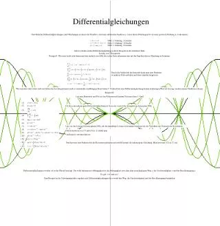
Vergleich zwischen Numerischer Differentialgleichung und Exakter Lösung Milot Mirdita
Numerik • Teilgebiet der Mathematik • Approximation • Anwendung • Wetterberechnung • Unfallsimulation • Wirtschaftsinformatik • … Milot Mirdita
Approximation, Fehler und Fehlerfortpflanzung • Problem: • Datentyp hat einen begrenzten Speicher • Unendliche Zahlenmenge muss auf eine endliche Zahlenmenge abgebildet werden. • Datentyp: • Fließkommazahlen (Float und Double) Milot Mirdita
Fließkommazahlen • Grundlage • Wissenschaftliche Notation: • c = 299.792.458 m/s • = 299.792,458 · 103 m/s • = 0,299792458 · 109 m/s • = 2,99792458 · 108 m/s r = m be Exponent Mantisse Basis Milot Mirdita
Beispiel • d = 50000; k1 = 0; k2 = 0; s0 = 0; v0 = 10; • t=0; tmax=50000; Milot Mirdita
Gedämpfte Harmonische Schwingungen FR V V Von Patrick FR= -Ds FD= -kv Fges= FR + FD ma = -Ds – kv ms(t) = -Ds(t) – ks(t) FD FD ∙ ∙ ∙ Gedämpfte Harmonische Schwingungen Fallunterscheidung Aperiodischer Grenzfall Herleitung 15
Numerisches Lösen der Schwingungsdifferentialgleichung • Gleichung: • Parameter • Anfangswert s0 und v0 • Koeffizienten: d, k1 und k2 • Schrittweite: h Milot Mirdita
Euler Cauchy Verfahren s(t + t) = s(t) + t s'(t) s'(t + t) = s'(t) + t s''(t) Milot Mirdita
Als Code while(t < t1) { y[0] = y[0] + h * y[1]; y[1] = y[1] + h * (-d * y[0] - k1 * y[1] + k2 * y[1] ^2); t = t + h; } Parameter: d=1; k1=0,1; k2=0; s0=0; v0=1; h=1; t=0; t1=5; Milot Mirdita
Schritt 1: while(0 < 5) { y[0] = 0 + 1 * 1; // 1 y[1] = 1 + 1 * (-1 * 0 – 0.1 * 1 + 0 * 1^2); // -0.99 t = 0 + 1; // 1 } Milot Mirdita
Schritt 2: while(1 < 5) { y[0] = 1 + (-0.99); // -0,0900000000000001 y[1] = (-0.99) + (-1 * 1 – 0.1 * (-0.99) + 0 * (-0.99)^2); // -0,801 t = 1 + 1; // 2 } Milot Mirdita
Schritt 3: while(2 < 5) { y[0] = -0,0900000000000001 + h * -0,801; // -0,891 y[1] = -0,801 + h * (-1 * -0,0900000000000001 – 0.1 * -0,801 + 0 * -0,801^2); //0,1701 t = 2 + 1; //3 } Milot Mirdita
Schritt 4: while(3 < 5) { y[0] = -0,891 + h * 0,1701; // -0,7209 y[1] = 0,1701 + h * (-1 * -0,891 – 0.1 * 0,1701 + 0 *0,1701^2); // 0,87399 t = 3 + 1; // 4 } Milot Mirdita
Schritt 5: while(4 < 5) { y[0] = -0,7209 + h * 0,87399; // 0,15309 y[1] = 0,87399 + h * (-1 * -0,7209 – 0.1 * 0,87399 + 0 *0,87399^2); // 0,633501 t = 4 + 1; //5 } Milot Mirdita
Graph Milot Mirdita
Verschiedene Schrittweiten Milot Mirdita
k2 (y’(x))2? pwind = cwρ/2 v2 y‘(x) = s‘(x) = v(x) Milot Mirdita
Ende!Fragen? Milot Mirdita