Download
1 / 61
610 likes | 747 Views
Segmentation. slides adopted from Svetlana Lazebnik. Segmentation as clustering. K-means clustering based on intensity or color is essentially vector quantization of the image attributes Clusters don’t have to be spatially coherent. Image. Intensity-based clusters. Color-based clusters.

E N D
Segmentation slides adopted from Svetlana Lazebnik
Segmentation as clustering • K-means clustering based on intensity or color is essentially vector quantization of the image attributes • Clusters don’t have to be spatially coherent Image Intensity-based clusters Color-based clusters
K-Means for segmentation • Pros • Very simple method • Converges to a local minimum of the error function • Cons • Memory-intensive • Need to pick K • Sensitive to initialization • Sensitive to outliers • Only finds “spherical” clusters
Mean shift clustering/segmentation • Find features (color, gradients, texture, etc) • Initialize windows at individual feature points • Perform mean shift for each window until convergence • Merge windows that end up near the same “peak” or mode
Mean shift segmentation results http://www.caip.rutgers.edu/~comanici/MSPAMI/msPamiResults.html
Mean shift pros and cons • Pros • Does not assume spherical clusters • Just a single parameter (window size) • Finds variable number of modes • Robust to outliers • Cons • Output depends on window size • Computationally expensive • Does not scale well with dimension of feature space
j wij i Segmentation by graph partitioning • Break Graph into Segments • Delete links that cross between segments • Easiest to break links that have low affinity • similar pixels should be in the same segments • dissimilar pixels should be in different segments A B C Source: S. Seitz
Measuring affinity • Suppose we represent each pixel by a feature vector x, and define a distance function appropriate for this feature representation • Then we can convert the distance between two feature vectors into an affinity with the help of a generalized Gaussian kernel:
Minimum cut • We can do segmentation by finding the minimum cut in a graph • Efficient algorithms exist for doing this Minimum cut example
Cuts with lesser weight than the ideal cut Ideal Cut Normalized cut • Drawback: minimum cut tends to cut off very small, isolated components * Slide from Khurram Hassan-Shafique CAP5415 Computer Vision 2003
Normalized cut • Drawback: minimum cut tends to cut off very small, isolated components • This can be fixed by normalizing the cut by the weight of all the edges incident to the segment • The normalized cut cost is: • w(A, B) = sum of weights of all edges between A and B • Solution to eigen decomposition of (D − W)y =λDy J. Shi and J. Malik. Normalized cuts and image segmentation. PAMI 2000
Challenge • How to segment images that are a “mosaic of textures”?
Using texture features for segmentation • Convolve image with a bank of filters J. Malik, S. Belongie, T. Leung and J. Shi. "Contour and Texture Analysis for Image Segmentation". IJCV 43(1),7-27,2001.
Using texture features for segmentation • Convolve image with a bank of filters • Find textons by clustering vectors of filter bank outputs Image Texton map J. Malik, S. Belongie, T. Leung and J. Shi. "Contour and Texture Analysis for Image Segmentation". IJCV 43(1),7-27,2001.
Using texture features for segmentation • Convolve image with a bank of filters • Find textons by clustering vectors of filter bank outputs • The final texture feature is a texton histogram computed over image windows at some “local scale” J. Malik, S. Belongie, T. Leung and J. Shi. "Contour and Texture Analysis for Image Segmentation". IJCV 43(1),7-27,2001.
An example Implemention • Compute an initial segmentation from the locally estimated weight matrix. a) Compute eigen-decomposition of Connectivity graph b) Pixel wise K-means with K=30 on the 11-dim subspace defined by the eigenvectors 2-12 c) Reduce K until error threshold is reached
An example Implemention • 1. Compute an initial segmentation from the locally estimated weight matrix. • 2. Update the weights using the initial segmentation. • - build histogram by considering pixels in the intersection of segmentation and local window
An example Implemention • 1. Compute an initial segmentation from the locally estimated weight matrix. • 2. Update the weights using the initial segmentation. • 3. Coarsen the graph with the updated weights to reduce the segmentation to a much simpler problem. • - Each segment is now a node in the graph • - Weights are computed through aggregation over the original graph matrix weights
An example Implementation • 1. Compute an initial segmentation from the locally estimated weight matrix. • 2. Update the weights using the initial segmentation. • 3. Coarsen the graph with the updated weights to reduce the segmentation to a much simpler problem. • 4. Compute a final segmentation using the coarsened graph. • 1. Compute the second smallest eigenvector for the generalized eigensystem using weights for coarsened graph • 2. Threshold the eigenvector to produce a bipartitioning of the image. 30 different values uniformly spaced within the range of the eigenvector are tried as the threshold. The one producing a partition which minimizes the normalized cut value is chosen. The corresponding partition is the best way to segment the image into two regions. • 3. Recursively repeat steps 1 and 2 for each of the partitions until the normalized cut value is larger than 0.1.
Results: Berkeley Segmentation Engine http://www.cs.berkeley.edu/~fowlkes/BSE/
Normalized cuts: Pro and con • Pros • Generic framework, can be used with many different features and affinity formulations • Cons • High storage requirement and time complexity • Bias towards partitioning into equal segments
Bottom-up segmentation Bottom-up approaches:Use low level cues to group similar pixels • Normalized cuts • Mean shift • …
Bottom-up segmentation is ill posed Many possible segmentation are equally good based on low level cues alone. Some segmentation example (maybe horses from Eran’s paper) images from Borenstein and Ullman 02
Top-down segmentation • Class-specific, top-down segmentation (Borenstein & Ullman Eccv02) • Winn and Jojic 05 • Leibe et al 04 • Yuille and Hallinan 02. • Liu and Sclaroff 01 • Yu and Shi 03
Combining top-down and bottom-up segmentation + • Find a segmentation: • Similar to the top-down model • Aligns with image edges
Why learning top-down and bottom-up models simultaneously? • Large number of freedom degrees in tentacles configuration- requires a complex deformable top down model • On the other hand: rather uniform colors- low level segmentation is easy
Combined Learning Approach • Learn top-down and bottom-up models simultaneously • Reduces at run time to energy minimization with binary labels (graph min cut)
Energy model Segmentation alignment with image edges Consistency with fragments segmentation
Energy model Segmentation alignment with image edges Consistency with fragments segmentation
Resulting min-cut segmentation Energy model Segmentation alignment with image edges Consistency with fragments segmentation
Learning from segmented class images Training data: Learn fragments for an energy function
Greedy energy design: Fragments selection Candidate fragments pool:
Results- horses dataset Mislabeled pixels percent Fragments number Comparable to previous but with far fewer fragments
Visual motion Many slides adapted from S. Seitz, R. Szeliski, M. Pollefeys
Motion and perceptual organization • Sometimes, motion is the only cue
Motion and perceptual organization • Sometimes, motion is foremost cue
Motion and perceptual organization • Even “impoverished” motion data can evoke a strong percept G. Johansson, “Visual Perception of Biological Motion and a Model For Its Analysis", Perception and Psychophysics 14, 201-211, 1973.
Motion and perceptual organization • Even “impoverished” motion data can evoke a strong percept G. Johansson, “Visual Perception of Biological Motion and a Model For Its Analysis", Perception and Psychophysics 14, 201-211, 1973.
Motion and perceptual organization • Even “impoverished” motion data can evoke a strong percept G. Johansson, “Visual Perception of Biological Motion and a Model For Its Analysis", Perception and Psychophysics 14, 201-211, 1973.
Uses of motion • Estimating 3D structure • Segmenting objects based on motion cues • Learning and tracking dynamical models • Recognizing events and activities
Motion field • The motion field is the projection of the 3D scene motion into the image
Motion field and parallax • X(t) is a moving 3D point • Velocity of scene point: V = dX/dt • x(t) = (x(t),y(t)) is the projection of X in the image • Apparent velocity v in the image: given by components vx = dx/dt and vy = dy/dt • These components are known as the motion field of the image X(t+dt) V X(t) v x(t+dt) x(t)
Motion field and parallax X(t+dt) To find image velocity v, differentiate x=(x,y) with respect to t (using quotient rule): V X(t) v x(t+dt) x(t) Image motion is a function of both the 3D motion (V) and thedepth of the 3D point (Z)