Download
1 / 81
860 likes | 1.26k Views
Segmentation. ECE 847: Digital Image Processing. Stan Birchfield Clemson University. What is segmentation?. Segmentation divides image(s) into groups over space and/or time Tokens are the things that are grouped (pixels, points, surface elements, etc.) Bottom-up segmentation:

E N D
Segmentation ECE 847:Digital Image Processing Stan Birchfield Clemson University
What is segmentation? • Segmentation divides image(s) into groups over space and/or time • Tokens are the things that are grouped (pixels, points, surface elements, etc.) • Bottom-up segmentation: • Tokens grouped because they share some local property (gray level, color, texture, motion, etc.) • Can be considered as either • segmentation / partitioningcarve dense data set into (disjoint) regionsor • grouping / clusteringgather sets of sparse items according to some model
Segmentation examples * * Pictures from Mean Shift: A Robust Approach toward Feature Space Analysis, by D. Comaniciu and P. Meer http://www.caip.rutgers.edu/~comanici/MSPAMI/msPamiResults.html
More examples from Pedro F. Felzenszwalb and Daniel P. Huttenlocher, Efficient Graph-Based Image Segmentation, IJCV, 59(2), 2004http://people.cs.uchicago.edu/~pff/segment/
Other examples • Shot detection • Figure / ground separation (background subtraction) • Collect tokens that lie on a line (robust line fitting) • Collect pixels that share the same fundamental matrix (independent 3D rigid motion)
Gestalt psychology Gestalt school of psychologists emphasized grouping as the key to understanding visual perception. Recall: Context affects how things are perceived gestalt – whole or group gestalt qualitat – set of internal relationships that makes it a whole Max Wertheimer, Laws of Organization in Perceptual Forms, 1923 http://psy.ed.asu.edu/~classics/Wertheimer/Forms/forms.htm
Gestalt psychology (cont.) Familiar configuration
Muller-Lyer illusion Lines are perceived as components of a whole rather than as individual lines.
3D interpretation of Muller-Lyer from http://www.michaelbach.de/ot/sze_muelue/
Illusory contours • Kanizsa triangle
Two final examples What role is top-down playing? from http://www-static.cc.gatech.edu/classes/AY2007/cs4495_fall/html/materials.html
Segmentation as partitioning • A partition of image is set of subsets S1, .., SN such that • I=U Si (covers entire image) • Si n Sj = 0 for all i != j (non-overlapping) • A predicate H(Si) measures region homogeneity • Segmentation seeks • H(Si) = true for all i • H(Si U Sj) = false for all adjacent Si, Sj
Region growing • Start with seed pixel • Repeat: • Accumulate neighboring pixels that are similar (according to some homogeneity criterion) • Algorithm is like floodfill, but homogeneity criterion is more complex • Grow multiple regions simultaneously, so no region dominates • Need to merge multiple regions
B Aa Ab Aa Ada Adc Add C D Region splitting • Start with entire image • Repeat: • Split any region that does not satisfy homogeneity criterion into subregions • Quad-tree representation is convenient • May need to merge regions that have been split
Split-and-Merge • Split-and-merge algorithm combines these two ideas • Split image into quadtree, where each region satisfies homogeneity criterion • Merge neighboring regions if their union satisfies criterion (like connected components) S. L. Horowitz and T. Pavlidis, Picture Segmentation by a Tree Traversal Algorithm, 1976
Split-and-merge results image after split after merge
Cluster together (pixels, tokens, etc.) that belong together Agglomerative clustering make each point a separate cluster repeat: merge two closest clusters Divisive clustering make a single cluster containing all points repeat: split cluster to yield two distant components (much harder) Segmentation as clustering • How to compute inter-cluster distance? • single-link clustering(dist. b/w closest elements) • complete-link clustering(dist. b/w farthest elements) • group-average clustering(use average distance) • Dendrograms • yield a picture of output as clustering process continues
Dendrograms raw data clusters represented as tree from http://en.wikipedia.org/wiki/Dendrogram
Watershed segmentation Interpret (gradient magnitude) image as topographical surface: watershedline catchment basin All pixels in catchment basin are connected to minimum by monotonically decreasing path
Watershed algorithms • Water immersion (Vincent-Soille) • Puncture hole at each local minimum, immerse in water • Grow level by level, starting with dark pixels • Sorting step: For efficiency, precompute for each graylevel a list of pixels with that graylevel (histogram with pointers) • Flooding step: Then, repeat: • Breadth-first search (floodfill) of level g given flooding up to level g-1 • For each pixel with value g, either assign to closest catchment basin or declare new catchment basin (geodesic influence zone) • Tobogganing • Find downstream path from each pixel to local minimum • Difficult to define for discrete (quantized) images because of plateaus
Vincent-Soille algorithm new basin created ≤ g-1 g multiple basins extended: decision chosen by breadth-first search basin extended
Watershed from Gonzalez and Woods, Digital Image Processing
Traditional watershed uses dams (But our implementation does not need dams)
Watershed results (But the results from our implementation will be better than this)
Marker-based watershed • Threshold image • Compute chamfer distance • Run watershed to get lines between objects • Set these lines (skeletons) and blobs to zero in the gradient image • Only allow new basins where the value is zero
Simplified Vincent-Soilles algorithm for marker-based marker[p] = true (FIFO queue is important – use std::deque)
Marker-based watershed edges threshold watershed chamfer image or markers gradient magnitude watershed
Why are ridges needed? threshold • Ridge markers define • background region • Without them, one object • will spill over into background • and disappear image markers gradient magnitude watershed
Another example image markers gradient magnitude watershed
Stochastic relaxation • Geman and Geman • Markov Random Field (MRF)
Region growing, balloons S. C. Zhu and A.L Yuille, Region Competition: Unifying Snake/balloon, Region Growing and Bayes/MDL/Energy for Multi-band Image Segmentation. IEEE Transactions on Pattern Analysis and Machine Intelligence, vol.18, no.9, pp.884-900, Sept. 1996.
Background subtraction Background subtraction provides figure-ground separation,which is a type of segmentation C. Wren et al., Pfinder: Real-Time Tracking of the Human Body http://vismod.media.mit.edu/vismod/demos/pfinder/
Represent tokens (which are associated with each pixel) using a weighted graph. affinity matrix (pij has affinity of 0) Cut up this graph to get subgraphs with strong interior links and weaker exterior links Graph theoretic clustering Application to vision originated with Shi and Malik at Berkeley
Graph Representations a b c e d Adjacency Matrix: W * From Khurram Hassan-Shafique CAP5415 Computer Vision 2003
Weighted Graphs a b c e 6 d Weight Matrix: W * From Khurram Hassan-Shafique CAP5415 Computer Vision 2003
Minimum Cut A cut of a graph G is the set of edges S such that removal of S from G disconnects G. Minimum cut is the cut of minimum weight, where weight of cut <A,B> is given as * From Khurram Hassan-Shafique CAP5415 Computer Vision 2003
Minimum Cut and Clustering * From Khurram Hassan-Shafique CAP5415 Computer Vision 2003
Image Segmentation & Minimum Cut Pixel Neighborhood w Image Pixels Similarity Measure Minimum Cut * From Khurram Hassan-Shafique CAP5415 Computer Vision 2003
Minimum Cut • There can be more than one minimum cut in a given graph • All minimum cuts of a graph can be found in polynomial time1. 1H. Nagamochi, K. Nishimura and T. Ibaraki, “Computing all small cuts in an undirected network. SIAM J. Discrete Math. 10 (1997) 469-481. * From Khurram Hassan-Shafique CAP5415 Computer Vision 2003
Finding the Minimal Cuts:Spectral Clustering Overview Data Similarities Block-Detection * Slides from Dan Klein, Sep Kamvar, Chris Manning, Natural Language Group Stanford University
Eigenvectors and Blocks • Block matrices have block eigenvectors: • Near-block matrices have near-block eigenvectors: [Ng et al., NIPS 02] 3= 0 1= 2 2= 2 4= 0 eigensolver 3= -0.02 1= 2.02 2= 2.02 4= -0.02 eigensolver * Slides from Dan Klein, Sep Kamvar, Chris Manning, Natural Language Group Stanford University
Spectral Space • Can put items into blocks by eigenvectors: • Resulting clusters independent of row ordering: e1 e2 e1 e2 e1 e2 e1 e2 * Slides from Dan Klein, Sep Kamvar, Chris Manning, Natural Language Group Stanford University
The Spectral Advantage • The key advantage of spectral clustering is the spectral space representation: * Slides from Dan Klein, Sep Kamvar, Chris Manning, Natural Language Group Stanford University
Clustering and Classification • Once our data is in spectral space: • Clustering • Classification * Slides from Dan Klein, Sep Kamvar, Chris Manning, Natural Language Group Stanford University
Measuring Affinity Intensity Distance Texture * From Marc Pollefeys COMP 256 2003
Scale affects affinity affinity matrix: Four isotropic Gaussians are sampled: eigenvalues: sdata=0.2 Four large eigenvalues