Download
1 / 40
420 likes | 563 Views
Segmentation. C. Phillips, Institut Montefiore, ULg, 2006. Definition. In image analysis, segmentation is the partition of a digital image into multiple regions (sets of pixels), according to some criterion.

E N D
Segmentation C. Phillips, Institut Montefiore, ULg, 2006
Definition In image analysis, segmentation is the partition of a digital image into multiple regions (sets of pixels), according to some criterion. The goal of segmentation is typically to locate certain objects of interest which may be depicted in the image. Segmentation criteria can be arbitrarily complex, and take into account global as well as local criteria. A common requirement is that each region must be connected in some sense.
A simple example of segmentation is thresholding a grayscale image with a fixed threshold t: each pixel p is assigned to one of two classes, P0 or P1, depending on whether I(p) < t or I(p) ≥ t. t=.5
Goal of brain image segmentation • Split the head volume into its « main » components: • gray matter (GM) • white matter (WM) • cerebrol-spinal fluid (CSF) • the rest/others • (tumour)
Segmentation approaches • Manual segmentation: • an operator classifies the voxels manually
Segmentation approaches • Semi-automatic segmentation: • an operator defines a set of parameters, that are passed to an algorithm Example: threshold at t=200
Segmentation approaches • Automatic segmentation: • no operator intervention • objective and reproducible
Intensity based segmentation Model the histogram of the image !
Segmentation - Mixture Model • Intensities are modelled by a mixture of K Gaussian distributions, parameterised by: • means • variances • mixing proportions
Compute belonging probabilities from Gaussian parameters Segmentation - Algorithm Starting estimates for belonging probabilities Compute Gaussian parameters from belonging probabilities Converged ? No Yes STOP
Segmentation - Problems Noise & Partial volume effect
Segmentation - Problems MR images are corrupted by a smooth intensity non-uniformity (bias). Intensity bias field Corrected image Image with bias artefact
Segmentation - Priors Overlay prior belonging probability maps to assist the segmentation • Prior probability of each voxel being of a particular type is derived from segmented images of 151subjects • Assumed to be representative • Requires initialregistration tostandard space.
Unified approach:segmentation-correction-registration • Bias correction informs segmentation • Registration informs segmentation • Segmentation informs bias correction • Bias correction informs registration • Segmentation informs registration
Unified Segmentation • The solution to this circularity is to put everything in the same Generative Model. • A MAP solution is found by repeatedly alternating among classification, bias correction and registration steps. • The Generative Model involves: • Mixture of Gaussians (MOG) • Bias Correction Component • Warping (Non-linear Registration) Component
Gaussian Probability Density • If intensities are assumed to be Gaussian of meanmkand variances2k,then the probability of a valueyiis:
Non-Gaussian Probability Distribution • A non-Gaussian probability density function can be modelled by a Mixture of Gaussians (MOG): Mixing proportion - positive and sums to one
Mixing Proportions • The mixing proportiongkrepresents the prior probability of a voxel being drawn from classk- irrespective of its intensity. • So:
Non-Gaussian Intensity Distributions • Multiple Gaussians per tissue class allow non-Gaussian intensity distributions to be modelled.
Probability of Whole Dataset • If the voxels are assumed to be independent, then the probability of the whole image is the product of the probabilities of each voxel: • It is often easier to work with negative log-probabilities:
Modelling a Bias Field • A bias field is included, such that the required scaling at voxeli,parameterised byb, isri(b). • Replace the means bymk/ri(b) • Replace the variances by(sk/ri(b))2
Modelling a Bias Field • After rearranging: y r(b) yr(b)
Tissue Probability Maps • Tissue probability maps (TPMs) are used instead of the proportion of voxels in each Gaussian as the prior. ICBM Tissue Probabilistic Atlases. These tissue probability maps are kindly provided by the International Consortium for Brain Mapping, John C. Mazziotta and Arthur W. Toga.
“Mixing Proportions” • Tissue probability maps for each class are available. • The probability of obtaining classkat voxeli, given weightsgis then:
Deforming the Tissue Probability Maps • Tissue probability images are deformed according to parametersa. • The probability of obtaining classkat voxeli, given weightsgand parametersais then:
The Extended Model • By combining the modifiedP(ci=k|q)and P(yi|ci=k,q), the overall objective function (E) becomes: The Objective Function
Optimisation • The “best” parameters are those that minimise this objective function. • Optimisation involves finding them. • Begin with starting estimates, and repeatedly change them so that the objective function decreases each time.
Schematic of optimisation Repeat until convergence... Holdg,m,s2andaconstant, and minimiseEw.r.t.b - Levenberg-Marquardt strategy, usingdE/dbandd2E/db2 Holdg,m,s2andbconstant, and minimiseEw.r.t.a - Levenberg-Marquardt strategy, usingdE/daandd2E/da2 Holdaandbconstant, and minimiseEw.r.t.g,mands2 -Use an Expectation Maximisation (EM) strategy. end (Iterated Conditional Mode)
Levenberg-Marquardt Optimisation • LM optimisation is used for the nonlinear registration and bias correction components. • Requires first and second derivatives of the objective function (E). • Parametersaandbare updated by • Increase lto improve stability (at expense of decreasing speed of convergence).
EM is used to update m, s2 and g For iteration (n), alternate between: • E-step: Estimate belonging probabilities by: • M-step: Set q(n+1) to values that reduce:
Hidden Markov Random Field • Voxels are NOT independent: • GM voxels are surrounded by other GM voxels, at least on one side. • Model the intensity and classification of the image voxels by 2 random field: • a visible field y for the intensities • a hidden field c for the classifications • Modify the cost function E: And, at each voxel, the 6 neighbouring voxels are used to to build Umrf, imposing local spatial constraints.
Hidden Markov Random Field T1 image T2 image
Hidden Markov Random Field T1 & T2: MoG + hmrf T1 only: MoG only White matter
Hidden Markov Random Field T1 & T2: MoG + hmrf T1 only: MoG only Gray matter
Hidden Markov Random Field T1 & T2: MoG + hmrf T1 only: MoG only CSF
Perspectives • Multimodal segmentation : • 1 image is good but 2 is better ! • Model the joint histogram using multi-dimensional normal distributions. • Tumour detection : • contrasted images to modify the prior images • automatic detection of outliers ?