Download
1 / 10
100 likes | 221 Views
Lecture 25 Radial Basis Network (II). Outline. Regularization Network Formulation Radial Basis Network Type 2 Generalized RBF network Training algorithm Implementation details. Properties of Regularization network. An RBF network is a universal approximator :

E N D
Outline • Regularization Network Formulation • Radial Basis Network Type 2 • Generalized RBF network • Training algorithm • Implementation details (C) 2001-2003 by Yu Hen Hu
Properties of Regularization network • An RBF network is a universal approximator: • it can approximate arbitrarily well any multivariate continuous function on a compact support in Rn where n is the dimension of feature vectors, given sufficient number of hidden neurons. • It is optimal in that it minimizes E(F). • It also has the best approximation property. That means given an unknown nonlinear function f, there always exists a choice of RBF coefficients that approximates f better than other possible choices of models. (C) 2001-2003 by Yu Hen Hu
Instead of xi, use virtual data points tjin the solution of F(x). Define Substitute each xi into eq. F(xi)=di we have a new system: (GTG + lGo)w = GTd Thus, w = (GTG + lGo)-1GTd when l = 0, w = G+d = (GTG)-1GTd where G+ is the pseudo-inverse matrix of G. Radial Basis Network (Type II) (C) 2001-2003 by Yu Hen Hu
RBN2 Algorithm Summary Given: {xi; 1 i K}, d: desired output, and J: # of radial basis neurons • Cluster {xi} into J clusters, find clustering centers {tj;1 j J}. Variance j2 or inverse covariance matrix j1 are also computed. • Compute G matrix (K by J) and G0 matrix. Gi,j+1 = exp(0.5||x(i)tj||2/j2) or Gi,j+1 = exp(0.5(x(i)tj)Tj1(x(i)tj)) Solve w = G†d or (GTG + lG0)-1GTd • Above procedure can be refined by fitting the clusters into a Gaussian mixture model and train it with the EM algorithm. (C) 2001-2003 by Yu Hen Hu
Example (C) 2001-2003 by Yu Hen Hu
Consider a Gaussian RBF model In RBN-II training, in order to compute {wi}, parameters {tj} are determined in advance using Kmeans clustering and s2is selected initially. To fit the model better at F(xi) = di, these parameters may need fine-tuning. Additional enhancements include Allowing each basis has its own width parameter sj, and A bias term is added to compensate for nonzero background value of the function over the support. While similar to the Gaussian mixture model, {wi} can be negative is the main difference. General RBF Network (C) 2001-2003 by Yu Hen Hu
The parameters q = {wj, tj, sj, b} are to be chosen to minimize the approximation error The steepest descent gradient method leads to: Specifically, for 1 m J Training of Generalized RBN (C) 2001-2003 by Yu Hen Hu
Note that Hence Thus, the individual parameters’ on-line learning formula are: Training … (C) 2001-2003 by Yu Hen Hu
The cost function may be augmented with additional smoothing terms for the purpose of regularization. For example, the derivative of F(x|q) may be bounded by a user-specified constant. However, this will make the training formula more complicated. Initialization of RBF centers and variance can be accomplished using the Kmeans clustering algorithm Selection of the number of RBF function is part of the regularization process and often need to be done using trail-and-error, or heuristics. Cross-validation may also be used to give a more objective criterion. A feasible range may be imposed on each parameter to prevent numerical problem. E.g. s2 e > 0 Implementation Details (C) 2001-2003 by Yu Hen Hu