Download

1 / 50
510 likes | 708 Views
A Min-max Cut Algorithm for Graph Partitioning and Data Clustering. Authors : Chris H.Q. Ding a , Xiaofeng He a,b , Hongyuan Zha b , Ming Gu c , Horst D. Simon a a NERSC Division, Lawrence Berkeley National Laboratory, University of California

E N D
A Min-max Cut Algorithm for Graph Partitioning and Data Clustering Authors : Chris H.Q. Dinga, XiaofengHea,b, HongyuanZhab, Ming Guc, Horst D. Simona aNERSC Division, Lawrence Berkeley National Laboratory, University of California bDepartment of Computer Science and Engineering, Pennsylvania State University cDepartment of Mathematics, University of California From : 1-th IEEE International Conference on Data Mining (ICDM), 2001 Google scholar : 419
Outline • 1. Introduction (5) • 2. Mix-max cut (11) • 3. Related work on spectral graph partition (5) • 4. Random graph model (2) • 5. Mcut algorithm (2) • 6. Experiments (5) • 7. Skewed cut (9) • 8. Linkage-based refinements (6) • 9. Linkage differential order (2) • 10. Conclusion
Introduction (1/5) • The graphs generated from the World Wide Web are highly irregular or random. • Partitioning the web graph is useful to automatically identify topics from the retrieved webpages for a user query.
Introduction (2/5) • In this paper, the authors emphasize graph partition as data clustering using a graph model. • Given the attributes of the data points in a dataset and the similarity or affinity metric between any two points, the symmetric forms a weighted adjacency matrix. • Thus, the data clustering problem becomes a graph partition problem.
Introduction (3/5) • The authors proposed a new graph partition method based on the min-max clustering principle : • The similarity or association between two subgraphs is minimized, while the similarity or association within each subgraph (summation of similarity between all pairs of nodes within a subgraph) is maximized.
Introduction (4/5) • The optimal solution to the graph partition problem is NP-complete. • The relaxed version of the min-max cut function optimization leads to a generalized eigenvalue problem.
Introduction (5/5) • The second lowest eigenvectors, also called the Fiedler vector, provides a linear search order (Fiedler vector) • It is generally believed that the Fiedler order provides the best known linearized order to search for the optimal cut. • Here, the authors find a linkage differential order that provides a better ordination than the Fiedler vector.
Min-max Cut (1/11) • Given a weighted graph G=G(E, V) and weight matrix W, we wish to partition it into two subgraphsA, B using the mix-max clustering principle. • The similarity or association between two nodes is their edge weight Wuv. • The similarity between subgraphsA, B is the cutsize.
Min-max Cut (2/11) The min-max clustering principle requires we minimize cut(A, B) while maximizing W(A) and W(B). All these requirements can be simultaneously satisfied by the following objective function : The authors called it the min-max cut function or Mcut for short.
Min-max Cut (3/11) • To reveal the solution, the authors reorder the rows and columns of Wconformally with subgraphsA and B such that
Min-max Cut (4/11) • Let x and y be vectors conformally partitioned with A and B. Mcut is invariant under changes of ||x||2 and ||y||2, and
Min-max Cut (6/11) Equation (7)
Min-max Cut (7/11) • It follows from Theorem 1 that both ratios of (7) are equal at the optimal solution : Hence the resulting clusters tend to have similar weights and are thus balanced.
Min-max Cut (8/11)Fiedler linear search order • The solution to partition problem can be represented by an indicator vector q, • where the nodal value of q on node u is qu = {a, -b}. • Theorem 1 implies that the solution vector x, y must lie in the eigenspace of . • The first eigenvector with the largest eigenvalue does not match q. • The second eigenvector z2 satisfies zT2z1=0 and has positive and negative elements. • A good approximation of q.
Min-max Cut (9/11)Fiedler linear search order • More directly, it can show that : Relaxing qu to real number in [-1, 1], the solution for minimizing Rayleigh quotientJN(q) is given by : subject to
Min-max Cut (10/11)Fiedler linear search order • We obtain the lower bound for the Mcut objective : Note that this bound is the same as the optimal Mcut value
Min-max Cut (11/11)Fiedler linear search order • 此節得到了三個結論 : • 1. 在適當的條件下,分群後的每群大小要相似。 • 2. 在適當的條件下,能夠找出最佳的近似解。 • 3. 在適當的條件下,能夠找出Mcut的lower bound.
Related work on spectral graph partition (1/5) • Spectral graph partitioning is based on the properties of eigenvectors of the Laplacian matrix L = D – W. • First developed by Donath and Hoffman [8] and Fiedler[11,12], and recently populated by the work of Pothen, Simon and Liu[21]. [8] Donath, W. E. and Homan, A. J. (1973). Lower bounds for the partitioning of graphs. IBM J. Res. Develop., 17, 420 - 425. [11] Fiedler, M. (1973). Algebraic connectivity of graphs. Czechoslovak Math. J., 23, 298 - 305. [12] M. Fiedler, A property of eigenvectors of nonnegative symmetric matrices and its application to graph theory, Czech. Math. J., 25, 619–637 (1975) [21]Pothen, A., Simon, H. D., and Liou, K. P. (1990). Partitioning sparse matrices with eigenvectors of graphs. SIAM Journal of Matrix Anal. Appl., 11, 430 - 452.
Related work on spectral graph partition (2/5) • The objective of the partitioning is to minimize the cut size J(A, B) = cut(A, B) with the requirement that two subgraphs have the same number of nodes : |A| = |B|.
Related work on spectral graph partition (3/5) • Hagen and Kahng [14] remove the requirement |A|=|B| and show that the Fiedler vector provides a good linear search order to the ratio cut (Rcut) partitioning criteria[4]. [4] C.-K. Cheng and Y.A. Wei. An improved two-way partitioning algorithm with stable performance. IEEE. Trans. on Computed Aided Design, 10: 1502-1511, 1991. [14] L. Hagen and A.B. Kahng. New spectral methods for ratio cut partitioning and clustering. IEEE. Trans. onComputed Aided Design, 11:1074-1085. 1992.
Related work on spectral graph partition (4/5) • Shi and Malik propose the normalized cut, • They show that Ncut can be reduced to Ncut(A, B) = JN(q). (Rayleigh quotient)
Related work on spectral graph partition (5/5) • Beside spectral partitioning methods, other recent partitioning methods seek to minimize the sum of subgraphdiameters, see [7] or k-center problem [1] for examples. [1] P.K. Agarwaland C.M. Procopiuc. Exact and approximation algorithms for clustering. Proc. 9th ACM- SIAMSymposium onDiscrete Algorithm, pages 658-667, 1998. [7] S. Doddi, M.V. Marathe, S. S. Ravi, D. S. Taylor, and P. Widmayer. Approximation algorithms for clustering to minimize the sum of diameters. Nordic Journal of Computing, 7(3):185, Fall 2000.
Random graph model (1/2) • Suppose we have a uniformly distributed random graph with n nodes. • For this random graph, any two nodes are connected with probability p . • The authors consider the four objective functions : • MINcut • Rcut • Ncut • Mcut
Random graph model (2/2) • It have the following • Theorem 2. • For random graphs, MINcut favors highly skewed cuts, i.e., very uneven sizes. • Mcutfavors balanced cut, i.e., both subgraphs have the same sizes. • Rcutand Ncut show no size preferences.
Mcut algorithm (1/2) • Step 1 : • Compute the Fiedler vector from Eq(10). • Sort nodal values to obtain the Fiedler order.
Mcut algorithm (2/2) • Step 2 : • Search for the optimal cut point corresponding to the lowest Mcut based on the Fiedler order. • Step 3 : • Do linkage-based refinements.
Experiments (1/5) • Here we perform experiments on newsgroup articles in 20 newsgroups. We focus on three datasets, each has two newsgroups:
Experiments (2/5) • Word-document matrix X is first constructed. • 2000 words are selected according to the mutual information between words and documents. • Tf-idfscheme for term weighting is used and standard cosine similarity between two documents. • When each document, column of X, is normalized to 1 using L2 norm, document-document similarities are calculated as W = XTX.
Experiments (3/5) • To increase statistics, the authors divide one newsgroup A randomly into K1 subgroups and the other newsgroup B randomly into K2subgraphs. • One of the K1 subgroups of A is mixed with one of the K2 subgroups of B to produce a dataset G. • The graph partition methods are run on this dataset G to produce two clusters. • This is repeated for all K1K2 pairs between A and B, and the accuracy is averaged.
Experiments (4/5) Balanced case. • Mcut performs about the same as Ncut for newsgroups NG1/NG2, where the cluster overlap is small. • Mcut performs better than Ncut for newsgroups NG10/NG11 and NG18/NG19, where the cluster overlap is large.
Experiments (5/5) Unbalanced case. • A harder problem due to the unbalanced prior distributions. • Mcut consistently performs better than Ncut for cases where the cluster overlaps are large.
Skewed cut (1/9) • Now study the reasons that Mcut consistently outperforms Ncut in large overlap cases. • Ncut can be written as :
*Ncut has two pronounced valleys, and produces a skewed cut, while Mcut has a very flat valley and gives balanced cuts.
Skewed cut (3/9) • Ncut produces a cutsize of 262.7, much larger than the weight W(B, B) = 169. • In the Mcutobjective, the cutsize is absent in the denominators; this provides a abalanced cut.
Skewed cut (4/9) • Prompted by these studies, the authors provide further analysis. • Consider the balanced cases where • Let : • f>0 is the average fraction of cut relative to within cluster associations.
Skewed cut (5/9) • A example of the f : • <W> = 100 • cutsize(A, B) = 50 • f = 50/100, = 0.5
Skewed cut (6/9) • The corresponding value is : • For a skewed partition A1, B1, we have W(A1)<<W(B1) and then cut(A1, B1)<<W(B1). The Ncut value is : 由於W(B1)太大造成後項近似於0,所以省略。
Skewed cut (7/9) • Using Ncut, a skewed or incorrect cut will happen if Ncut1<Ncut0 :
Skewed cut (8/9) • Repeat the same analysis using Mcut : • For large overlap case, say, f=1/2, the condition for possible skewed cut are : 上面這兩個條件,是在認為skewed partition的情況底下所推論出來的式子。
Skewed cut (9/9) • The condition for skewed Ncut is satisfied most of the time, leading to many skewed cuts and there lower clustering accuracy. • Mcut is not satisfied most of the time, leading to more correct cuts and therefore higher clustering accuracy.
Linkage-based refinements (1/6) • The linear search order provided by sorting the Fiedler vector q implies that nodes on one side of the cut point must belong to one cluster :
Linkage-based refinements (2/6) • How to identify those nodes near the cut? • For this purpose, the authors define linkage l between two subgraphs :
Linkage-based refinements (3/6) • For a single node u, its linkage to subgraph A is : • If u is well inside a cluster, u will have a large linkage with the cluster. • If u is near the cut, its linkages with both clusters should be close. • Therefore, the authors define the linkage difference :
Linkage-based refinements (4/6) The cut point. • The authors move all nodes in cluster A with negative value to cluster B if the objective function is lowered. • This procedure of swapping nodes is called the “linkage-based swap.”
Linkage-based refinements (5/6) • The greedy move starts from the top of the list to the last node u where s(u)∆l(u)≥0. • s(u)=-1 if u belongs to A. • s(u)=1 if u belongs to B. • If s(u)∆l(u)<0 but close to 0, node u is in the correct cluster, although it is close to the cut. • Select the smallest 5% of the nodes with s(u)∆l(u)<0 as the candidates. • Move those which reduce Mcut objective to the other cluster. • Called this procedure “linkage-based move.”
Linkage differential order (1/2) • Given the linkage difference in Figure 2, we see that quite a few nodes far away from the cut point have wrong ∆l signs, that is, they belong to the other subgraph. • This strongly suggests that the Fiedler order is not necessarily the best linear search order.
Linkage differential order (2/2) • We can sort linkage difference ∆l to obtain a linear order different from the Fiedler order, which will be referred to as linkage differential (LD) order.
Conclusion • 1. Introduce the Mcut algorithm for graph partition. • 2. Shows that min-max objective function follows the clustering principle and produces balanced partitions. • 3. The linkage difference metric effectively identifies those nodes near the cut. • 4. The new linkage differential order is shown to provide a better linear search order than the best known Fiedler order.