V15: Max-Flow Min-Cut

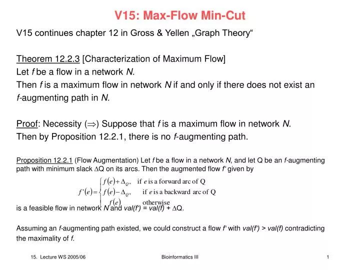
1. V15: Max-Flow Min-Cut V15 continues chapter 12 in Gross & Yellen „Graph Theory“ Theorem 12.2.3 [Characterization of Maximum Flow] Let f be a flow in a network N. Then f is a maximum flow in network N if and only if there does not exist an f-augmenting path in N. Proof: Necessity () Suppose that f is a maximum flow in network N. Then by Proposition 12.2.1, there is no f-augmenting path. Proposition 12.2.1 (Flow Augmentation) Let f be a flow in a network N, and let Q be an f-augmenting path with minimum slack Q on its arcs. Then the augmented flow f‘ given by is a feasible flow in network N and val(f‘) = val(f) + Q. Assuming an f-augmenting path existed, we could construct a flow f‘ with val(f‘) > val(f) contradicting the maximality of f. Bioinformatics III

2. V15: Max-Flow Min-Cut Sufficiency () Suppose that there does not exist an f-augmenting path in network N. Consider the collection of all quasi-paths in network N that begin with source s, and let Vs be the union of the vertex-sets of these quasi-paths. Since there is no f-augmenting path, it follows that sink t  Vs. Let Vt = VN – Vs. Then Vs,Vt is an s-t cut of network N. Moreover, by definition of the sets Vsand Vt , Hence, f is a maximum flow, by Corollary 12.1.8. □ Bioinformatics III

3. V15: Max-Flow Min-Cut Theorem 12.2.4 [Max-Flow Min-Cut] For a given network, the value of a maximum flow is equal to the capacity of a minimum cut. Proof: The s-t cut constructed in the proof of Theorem 12.2.3 has capacity equal to the maximum flow. □ The outline of an algorithm for maximizing the flow in a network emerges from Proposition 12.2.1 and Theorem 12.2.3. Bioinformatics III

4. Finding an f-Augmenting Path The discussion of f-augmenting paths culminating in the flow-augmenting Proposition 12.2.1 provides the basis of a vertex-labeling strategy due to Ford and Fulkerson that finds an f-augmenting path, when one exists. Their labelling scheme is essentially basic tree-growing. The idea is to grow a tree of quasi-paths, each starting at source s. If the flow on each arc of these quasi-paths can be increased or decreased, according to whether that arc is forward or backward, then an f-augmenting path is obtained as soon as the sink t is labelled. A frontier arc is an arc e directed from a labeled endpoint v to an unlabeled endpoint w. For constructing an f-augmenting path, the frontier path e is allowed to be backward (directed from vertex w to vertex v), and it can be added to the tree as long as it has slack e > 0. Bioinformatics III

5. Finding an f-Augmenting Path Terminology: At any stage during tree-growing for constructing an f-augmenting path, let e be a frontier arc of tree T, with endpoints v and w. The arc e is said to be usable if, for the current flow f, either e is directed from vertex v to vertex w and f(e) < cap(e), or e is directed from vertex w to vertex v and f(e) > 0. Frontier arcs e1 and e2 are usable if f(e1) < cap(e1) and f(e2) > 0 Remark From this vertex-labeling scheme, any of the existing f-augmenting paths could result. But the efficiency of Algorithm 12.2.1 is based on being able to find „good“ augmenting paths. If the arc capacities are irrational numbers, then an algorithm using the Ford&Fulkerson labeling scheme might not terminate (strictly speaking, it would not be an algorithm). Bioinformatics III

6. Finding an f-Augmenting Path Even when flows and capacities are restricted to be integers, problems concerning efficiency still exist. E.g., if each flow augmentation were to increase the flow by only one unit, then the number of augmentations requred for maximization would equal the capacity of a minimum cut. Such an algorithm would depend on the size of the arc capacities instead of on the size of the network. Bioinformatics III

7. Finding an f-Augmenting Path Example: For the network shown below, the arc from vertex v to vertex w has flow capacity 1, while the other arcs have capacity M, which could be made arbitrarily large. If the choice of the augmenting flow path at each iteration were to alternate between the directed path  s,v,w,t  and the quasi path  s,w,v,t , then the flow would increase by only one unit at each iteration. Thus, it could take as many as 2M iterations to obtain the maximum flow. Bioinformatics III

8. Finding an f-Augmenting Path Edmonds and Karp avoid these problems with this algorithm. It uses breadth-first search to find an f-augmenting path with the least number of arcs. Bioinformatics III

9. FFEK algorithm: Ford, Fulkerson, Edmonds, and Karp Algorithm 12.2.3 combines Algorithms 12.2.1 and 12.2.2 Bioinformatics III

10. FFEK algorithm: Ford, Fulkerson, Edmonds, and Karp Example: the figures illustrate algorithm 12.2.3. shown is s-t cut with capacity equal to the current flow, establising optimality. Bioinformatics III

11. FFEK algorithm: Ford, Fulkerson, Edmonds, and Karp At the end of the final iteration, the arc directed from source s to vertex w and the arc directed from vertex v to sink t are the only frontier arcs of the tree T, but neither is usable. These two arcs from the minimum cut  {s,x,y,z,v }, {w,a,b,c,t} . This illustrates the s-t cut that was constructed in the proof of theorem 12.2.3. Bioinformatics III

12. Determining the connectivity of a graph In this section, we use the theory of network flows to give constructive proofs of Menger‘s theorem. These proofs lead directly to algorithms for determining the edge-connectivity and vertex-connectivity of a graph. Strategy to prove Menger‘s theorems is based on properties of certain networks whose arcs all have unit capacity. These 0-1 networks are constructed from the original graph. Bioinformatics III

13. Determining the connectivity of a graph Lemma 12.3.1. Let N be an s-t network such that outdegree(s) > indegree(s), indegree(t) > outdegree (t), and outdegree(v) = indegree(v) for all other vertices v. Then, there exists a directed s-t path in network N. Proof. Let W be a longest directed trail (trail = walk without repeated edges; path = trail without repeated vertices) in network N that starts at source s, and let z be its terminal vertex. If vertex z were not the sink t, then there would be an arc not in trail W that is directed from z (since indegree(z) = outdegree(z) ). But this would contradict the maximality of trail W. Thus, W is a directed trail from source s to sink t. If W has a repeated vertex, then part of W determines a directed cycle, which can be deleted from W to obtain a shorter directed s-t trail. This deletion step can be repeated until no repeated vertices remain, at which point, the resulting directed trail is an s-t path. □ Bioinformatics III

14. Determining the connectivity of a graph Proposition 12.3.2. Let N be an s-t network such that outdegree(s) – indegree(s) = m = indegree(t) – outdegree (t), and outdegree(v) = indegree(v) for all vertices v  s,t. Then, there exist m disjoint directed s-t path in network N. Proof. If m = 1, then there exists an open eulerian directed trail T from source s to sink t by Theorem 6.1.3. Review: An eulerian trail in a graph is a trail that contains every edge of that graph. Theorem 6.1.3. A connected digraph D has an open eulerian trail from vertex x to vertex y if and only if indegree(x) + 1 = outdegree(x), indegree(y) = outdegree(y) + 1, and all vertices except x and y have equal indegree and outdegree. Theorem 1.5.2. Every open x-y walk W is either an x-y path or can be reduced to an x-y path. Therefore, trail T is either an s-t directed path or can be reduced to an s-t path. Bioinformatics III

15. Determining the connectivity of a graph By way of induction, assume that the assertion is true for m = k, for some k  1, and consider a network N for which the condition holds for m = k +1. There exists a directed s-t path P by Lemma 12.3.1. If the arcs of path P are deleted from network N, then the resulting network N satisfies the condition of the proposition for m = k. By the induction hypothesis, there exist k arc-disjoint directed s-t paths in network N. These k paths together with path P form a collection of k + 1 arc-disjoint directed s-t paths in network N. □ Bioinformatics III

16. Basic properties of 0-1 networks Definition A 0-1 network is a capacitated network whose arc capacities are either 0 or 1. Proposition 12.3.3. Let N be an s-t network such that cap(e) = 1 for every arc e. Then the value of a maximum flow in network N equals the maximum number of arc-disjoint directed s-t paths in N. Proof: Let f* be a maximum flow in network N, and let r be the maximum number of arc-disjoint directed s-t paths in N. Consider the network N* obtained by deleting from N all arcs e such that f*(e) = 0. Then f*(e) = 1 for all arcs e in network N*. It flollows from the definition that for every vertex v in network N*, and Bioinformatics III

17. Basic properties of 0-1 networks Thus by the definition of val(f*) and by the conservation-of-flow property, outdegree(s) – indegree (s) = val(f*) = indegree(t) – outdegree(t) and outdegree(v) = indegree(v), for all vertices v  s,t. By Proposition 12.3.2., there are val(f*) arc-disjoint s-t paths in network N*, and hence, also in N, which implies that val(f*)  r. To obtain the reverse inequality, let {P1,P2, ..., Pr} be the largest collection of arc-disjoint directed s-t paths in N, and consider the function f: EN  R+defined by Then f is a feasible flow in network N, with val(f) = r. It follows that val(f*)  r. □ Bioinformatics III

18. Separating Sets and Cuts Review from §5.3 Let s and t be distinct vertices in a graph G. An s-t separating edge set in G is a set of edges whose removal destroys all s-t paths in G. Thus, an s-t separating edge set in G is an edge subset of EG that contains at least one edge of every s-t path in G. Definition: Let s and t be distinct vertices in a digraph D. An s-t separating arc set in D is a set of arcs whose removal destroys all directed s-t paths in D. Thus, an s-t separating arc set in D is an arc subset of ED that contains at least one arc of every directed s-t path in digraph D. Remark: For the degenerate case in which the original graph or digraph has no s-t paths, the empty set is regarded as an s-t separating set. Bioinformatics III

19. Separating Sets and Cuts Proposition 12.3.4 Let N be an s-t network such that cap(e) = 1 for every arc e. Then the capacity of a minimum s-t cut in network N equals the minimum number of arcs in an s-t separating arc set in N. Proof: Let K* = Vs ,Vt be a minimum s-t cut in network N, and let q be the minimum number of arcs in an s-t separating arc set in N. Since K* is an s-t cut, it is also an s-t separating arc set. Thus cap(K*)  q. To obtain the reverse inequality, let S be an s-t separating arc set in network N containing q arcs, and let R be the set of all vertices in N that are reachable from source s by a directed path that contains no arc from set S. Then, by the definitions of arc set S and vertex set R, t  R, which means that  R, VN - R  is an s-t cut. Moreover,  R, VN - R  S. Therefore Bioinformatics III

20. Separating Sets and Cuts which completes the proof. □ Bioinformatics III

21. Arc and Edge Versions of Menger’s Theorem Revisited Theorem 12.3.5 [Arc form of Menger‘s theorem] Let s and t be distinct vertices in a digraph D. Then the maximum number of arc-disjoint directed s-t paths in D is equal to the minimum number of arcs in an s-t separating set of D. Proof: Let N be the s-t network obtained by assigning a unit capacity to each arc of digraph D. Then the result follows from Propositions 12.3.3. and 12.3.4., together with the max-flow min-cut theorem. □ Remark The edge form of Menger‘s theorem for undirected graphs follows directly from the next two assertions concerning the relationship between a graph G and the digraph obtained by replacing each edge e of graph G with a pair of oppositely directed arcs having the same endpoints as edge e. Each of these assertions follows directly from the definitions. Bioinformatics III

22. Arc and Edge Versions of Menger’s Theorem Revisited Assertion 12.3.6. Let s and t be distinct vertices of a graph G, and let be the digraph obtained by replacing each edge e of G with a pair of oppositely directed arcs having the same endpoints as edge e. Then there is a one-to-one correspondence between the s-t paths in graph G and the directed s-t paths in digraph . Moreover, two s-t paths in graph G are edge-disjoint if and only if their corresponding directed s-t paths in digraph are arc-disjoint. Assertion 12.3.7. Let s and t be distinct vertices of a graph G, and let be defined as above. Then the minimum number of edges in an s-t separating set of graph G is equal to the minimum number of arcs in an s-t separating arc set of digraph . Bioinformatics III

23. Arc and Edge Versions of Menger’s Theorem Revisited Theorem 12.3.8 [Edge form of Menger‘s theorem]. Let s and t be distinct vertices in a graph G. Then the maximum number of edge-disjoint s-t paths in G equals the minimum number of edges in an s-t separating edge set of graph G. Proof: This is an immediate consequence of Assertions 12.3.6 and 12.3.7, together with the arc form of Menger‘s theorem (theorem 12.3.5). Review from §5.1 The edge-connectivity e(G) is the size of a smallest edge-cut in graph G. Definition Let s and t be distinct vertices in a graph G. The local edge-connectivity between vertices s and t , denoted e(s,t) is the minimum number of edges in an s-t separating edge set in G. Bioinformatics III

24. Determining Edge-Connectivity Using Network Flows Proposition 12.3.9 The edge-connectivity of a graph G is equal to the minimum of the local edge-connectivites, taken over all pairs of vertices s and t. That is: Proposition 12.3.9 and theorem 12.3.8 suggest an algorithm for determining the edge-connectivity e(G) of an arbitrary graph G. The algorithm calculates the local edge-connectivity between each pair of vertices in G, by solving an appropriate maximum flow problem in the network . In fact, as the next two results show, it is not necessary to calculate the local edge-connectivity between every pair of vertices. Bioinformatics III

25. Determining Edge-Connectivity Using Network Flows Proposition 12.3.10. Let V1,V2 be a partition-cut of minimum cardinality in a graph G, and let v1 and v2 be any vertices in V1 and V2, respectively. Then the edge-connectivity e(G) equals the local edge-connectivity e(v1,v2). Proof: Suppose that the minimum local edge-connectivity is achieved between vertices x and y. Then e(G)  e(x,y)by Proposition 12.3.9. It suffices to show that e(v1,v2)  e(x,y). Let be the digraph obtained by replacing each edge of graph G with two oppositely directed arcs. Then can be regarded as a v1-v2 capacitated network and as an x-y capacitated network where each arc is assigned unit capacity. Let K* be a minimum v1-v2cut in network Bioinformatics III

26. Determining Edge-Connectivity Using Network Flows It follows that cap(K*)  cap  V1,V2 , since the partition-cut  V1,V2  corresponds to a v1-v2cut in network . Next, let f* be a maximum flow and V1 ,V2 a minimum x-y cut in x-y network so that cap(Vx,Vy) = val(f*). Then □ Bioinformatics III

27. Arc and Edge Versions of Menger’s Theorem Revisited Corollary 12.3.11 Let s be any vertex in a graph G. Then Proof: Let V1 ,V2  be a partition-cut of minimum cardinality, and suppose, without loss of generality, that vertex s  V1. There must be some vertex t  V2(otherwise, EG = , and the assertion would be trivially true). By Proposition 12.3.10 it follows that e(G) = e(s,t). □ The variable eused in the next algorithm, represents the edge-connectivity of graph G and is initialized with the sufficiently large positive integer |EG|. Bioinformatics III

28. Arc and Edge Versions of Menger’s Theorem Revisited Algorithm 12.3.1 requires O(n) iterations, and since Algorithm 12.2.3 requires O(n|E|2) computations, the overall complexity of algorithm 12.3.1 is O(n2|E|2). More efficient algorithms exist. Bioinformatics III

29. Using Network Flows to Prove the Vertex Forms of Menger’s Theorem Construction of Digraph ND from Digraph D. Let s and t be any pair of non-adjacent vertices in a digraph D. The digraph NDis obtained from digraph D as follows: - each vertex x  VD – {s,t} corresponds to two vertices x‘ and x‘‘ in digraph ND and an arc directed from x‘ to x‘‘. - each arc in digraph D that is directed from vertex s to vertex x  VD – {s,t} corresponds to an arc in NDdirected from s to x‘. - each arc in D that is directed from a vertex x  VD – { s,t } to vertex t corresponds to an arc in NDdirected from x‘‘ to t. - each arc in D that is directed from a vertex x  VD – {s,t} to a vertex y  VD – {s,t} corresponds to an arc in ND directed from x‘‘ to y‘. Bioinformatics III

30. Using Network Flows to Prove the Vertex Forms of Menger’s Theorem Review from §5.3: Let s and t be a pair of non-adjacent vertices in a graph G (or digraph D). An s-t separating vertex set in G (or in D) is a set of vertices whose removal destroys all s-t paths in G (or all directed s-t paths in D). Thus, an s-t separating vertex set is a set of vertices that contains at least one internal vertex of every (directed) s-t path. Definition Two (directed) s-t paths in a digraph D are internally disjoint if they have no internal vertices in common. Bioinformatics III

31. Relationship between digraphs D and ND Assertion 12.3.12 There is a one-to-one correspondence between directed s-t paths in digraph D and directed s-t paths in digraph ND. Assertion 12.3.13 Two directed s-t paths in D are internally disjoint if and only if their corresponding s-t directed paths in ND are arc-disjoint. Assertion 12.3.14 The maximum number of internally disjoint directed s-t paths in D is equal to the maximum number of arc-disjoint directed s-t paths in ND. Assertion 12.3.15 The minimum number of vertices in an s-t separating vertex set in digraph D is equal to the minimum number of arcs in an s-t separating arc set in digraph ND. Bioinformatics III

32. Relationship between digraphs D and ND Theorem 12.3.16 [Vertex Form of Menger for Digraphs] Let s and t be a pair of non-adjacent vertices in a digraph D. Then the maximum number of internally disjoint directed s-t paths in D is equal to the minimum number of vertices in an s-t separating vertex set in D. Proof: This follows from Assertions 12.3.12 through 12.3.15 together with the arc form of Menger‘s theorem (theorem 12.3.5). Theorem 12.3.17 [Vertex Form of Menger for Undirected Graphs]. Let s and t be a pair of non-adjacent vertices in a graph G. Then the maximum number of internally disjoint s-t paths in G is equal to the minimum number of vertices in an s-t separating vertex set in G. Proof: This follows from Theorem 12.3.16 and Assertions 12.3.6 and 12.3.7. Bioinformatics III

33. Determining Vertex-Connectivity using Network Flow Review from §5.3: Let s and t be non-adjacent vertices of a connected graph G. Then the local vertex-connectivity between s and t, denoted v(s,t) is the minimum number of vertices in an s-t separating vertex set. Lemma 5.3.5. Let G be a connected graph containing at least one pair of non-adjacent vertices. Then the vertex connectivity v(G) is the minimum of the local vertex-connectivity v(s,t), taken over all pairs of non-adjacent vertices s and t. The following algorithm, with O(n|EG|3) time-complexity, computes the vertex-connectivity of an n-vertex graph by calculating the local vertex-connectivity between various pairs of non-adjacent vertices. As in algorithm 12.3.1, it is not necessary to calculate the local vertex-connectivity between each pair. Bioinformatics III

34. Determining Vertex-Connectivity using Network Flow Bioinformatics III