Download
1 / 14
140 likes | 299 Views
Chapter 5 LR Demand for Labor. Long run (LR): period of time that is long enough for firm to vary both K and L (in response to es in: factor prices/demand, technology). Decision: pick K/L combo to produce Q at minimum cost; based on two factors:

E N D
Chapter 5LR Demand for Labor • Long run (LR): period of time that is long enough for firm to vary both K and L (in response to es in: factor prices/demand, technology). • Decision: pick K/L combo to produce Q at minimum cost; based on two factors: • 1. Substitutability of K and L: given by production function. • 2. Relative prices of K and L.
Production Function • Shows technological constraints. • Relationship between es in K and L and es in Q; • Also shows how can K and L keeping Q constant. • Isoquant: “iso” means same. • Shows substitutability between K and L, keeping Q fixed. • MRTS: marginal rate of technical substitution: measures the reduction in K needed if labor is by one unit and Q held fixed. • Convex: MRTS diminishes as move down isoquant.
Fixed Proportions Production Function • Only one combination of K and L can be used to produce each Q level. • No substitutability (MRTS=0). • Only relevant points are the “corner” points, with least-cost combination of K/L for each Q shown as line from origin thru these corner points.
Factor Prices • Price of labor = wage = w. • Price of capital = “rental rate” of K = r. • Isocost line: given factor prices, shows all combinations of K and L that firm could purchase with specific $ expenditure = E. • Given E1: • If only buy L: E1/w1 = L1 units. • If only buy K: E1/r1 = K1 units.
Features of Isocost Line • 1. Slope = -w1/r1 = constant. • (Derive with rise/run, where the E1 cancel.) • 2. For given factor prices: if E shift isocost parallel to right (no slope). • 3. If K or L slope (so an intercept changes). • Example: If w w/r; so steeper isocost line; es horizontal intercept.
Cost-Minimizing Employment Level • Assume for now: already know the firm’s profit-maximizing Q level (where P=MC); so given this Q*, pick K/L combo. • Cost-minimizing K/L combo: Occurs at tangency: where slope of isocost = slope of isoquant; • MRTS = -w/r. • Equilibrium condition: rate that technology says K/L can be traded off equals rate market says K/L can be traded off (based on factor price ratio).
Firm’s Profit-Max Choice of Q* • Firm picks Q* at point where the market price equals MC of production; P = MC. • Price line is horizontal line; also referred to as Demand curve (perfectly competitive firm faces perfectly elastic D curve since it can sell all it wants to at market P). • If w, MC too (MC shifts).
Firm Makes Two Distinct Decisions • Decision #1: profit-maximizing choice of output = Q*. • Decision #2: given this Q*, cost-minimizing choice of K and L. • Effect of wage: • 1. Shifts MC curve so es Q*. • 2. (w/r) so pivots isocost line; so es horizontal intercept too.
Effect of Wage on Firm’s Desired Employment Level • Key: w for just this firm. • Remember: wage affects choice of Q* first, then affects choice of K and L. • wage: shifts MC curve to left Q*. • Since Q*, must be on isoquant farther to left. • This w is a (w/r) so isocost line gets steeper (pivot to left around same vertical intercept). • See will change both K and L in LR.
LR Demand Curve for Labor • Connect the two long run points from previous example. • Note: LR DL curve is flatter (more elastic) than SR DL curve because in the LR, the firm has more chances of substitution since K is not fixed. • In LR: DL is more responsive to wage changes.
Determinants of Elasticity of DL • Why care? • Helps to predict employment effects of various policies: • wage subsidy. • unions pushing for higher wages. • increase in minimum wage.
Four Laws of Derived Demand • DL will be more elastic (ceteris paribus): • 1) the larger the price elasticity of demand for the product. • 2) the greater the share of labor cost as a percentage of TC. • 3) the greater the ease of substitution in production between K and L. • 4) the greater the elast of S of other competing factors like K.
Technological Change and Labor Demand • Remember: technological change will result in entirely new production function. • Technological change has two effects on employment; net impact depends on which is bigger: • 1) DL: better technology allows firms to produce given Q with fewer workers. • 2) DL: better technology costs of production product prices and product sales. • In general: winners and losers.
Displaced Workers • Issue: Even if technological change leads to overall increase in employment, some workers lose jobs. • These workers referred to as displaced workers. • Policies include: • 1) regular UI. • 2) targeted training programs. • 3) legislation requiring advance notice of mass layoffs.