Download

1 / 55
550 likes | 803 Views
Chapter 5 Models for Uncertain Demand. Aims of the chapter. Introduce uncertainty and develop some models where are not known exactly but follow known probability distributions. In particular, we focus on variable demand. Uncertainty in stocks. Areas with uncertainty

E N D
Aims of the chapter • Introduce uncertainty and develop some models where are not known exactly but follow known probability distributions. • In particular, we focus on variable demand.
Uncertainty in stocks Areas with uncertainty • The models we developed in the last chapter assumed that costs, demand, lead time and all other variables are known exactly. In other words, there is no uncertainty about the stocks. • In practice, there is almost always some uncertainty in stocks - as prices rise with inflation, operations change, new products become available, supply chains are disrupted, competition alters, new laws are introduced, the economy varies, customers and suppliers move, and so on.
From an organization's point of view, the main uncertainty is likely to be in customer demand, which might appear to fluctuate randomly or follow some long-term trend. • In this chapter we will develop some models to deal with this uncertainty.
What we mean by “uncertainty” • For inventory management this means that a value is not known exactly, but follows a known probability distribution. • Long-term demand for a product might, for example, be Normally distributed with a mean of 10 units a week and variance of 2 units a week. We cannot say exactly what demand in a particular week will be, but know that it is a figure drawn from this distribution.
We can classify problems according to variables that are: • unknown - in which case we have complete ignorance of the situation and any analysis is difficult; • known (and either constant or variable) - in which case we know the values taken by parameters and can use deterministic models; • uncertain - in which case we have probability distributions for the variables and can use probabilistic or stochastic(隨機的 ) models.
You can find uncertainty in many aspects of stock. Sometimes this is due to internal operations. No matter how good the operations are, there is always some variation that can lead to uncertainty. • Differences in materials, weather, tools, employees, moods(情緒 ), time, stress, and a whole range of other things combine to give apparently random variations. • The traditional way of dealing with these was to set a tolerance(公差 ) in the specifications.
Provided performance is within a specified range it is considered acceptable. • A 250 g bar of chocolate might weigh between 249.9 g and 250.1 g and still be considered the right weight; a train might arrive within ten minutes of its published time and still be considered on time. • Performance was only considered to be a problem when it fell outside the tolerance.
Taguchi (1986) pointed out that this approach has an inherent weakness. • Suppose a bank sets the acceptable time to open a new account as between 20 and 30 minutes. If the time taken is 20, 25 or 30 minutes, the traditional view says that these are equally acceptable - the process is achieving its target so there is no need for improvement. • But customers would probably not agree that taking 30 minutes is as good as taking 20 minutes. On the other hand, there might be little real difference between taking 30 minutes (which is acceptable) and 31 minutes (which is unacceptable).
However, there is still some variability that comes from external causes and the organization cannot control it. • Every organization works within a context that is set by international trading conditions, the national economy, government policies, the business environment, competition, other organizations in the supply chain, suppliers operations, and so on.
An organization cannot change these, but they are likely to affect several areas Demand. • Aggregate demand for an item usually comes from a number of separate customers. The organization has little real control over who buys their products, or how many they buy. Random fluctuations in the number and size of orders give a variable and uncertain overall demand.
Costs • Most costs tend to drift upwards with inflation, and we cannot predict the size and timing of increases. On top of this underlying trend, are short-term variations caused by changes to operations, products, suppliers, competitors, and so on. • Another point - that we mentioned in Chapter 2 - is that changing the accounting conventions can change the apparent costs.
Lead time • Lead time. There can be many stages between the decision to buy an item and actually having it available for use. Some variability in this chain is inevitable, especially if the item has to be made and shipped over long distances. A hurricane in the Atlantic, or earthquake in southern Asia can have surprisingly far-reaching effects on trade.
Deliveries • Orders are placed for a certain number of units of a specified item, but there are times when these are not actually delivered. • The most obvious problem is a simple mistake in identifying an item or sending the right number. • Other problems include quality checks that reject some delivered units, and damage or loss during shipping. • On the other hand, a supplier might allow some overage and send more units than requested. The deliveries ultimately depend on - and define - supplier reliability.
Overall, the key issue for probabilistic models is the lead time demand. • It does not really matter what variations there are outside the lead time, as we can allow for them by adjusting the timing and size of the next order. • Once we have placed an order, though, and are working within the lead time it is too late to make any adjustments.
If demand outside the lead time is higher than expected, all that happens is that we reach the reorder level sooner than expected: • but if demand inside the lead time is higher than expected, it is too late to make adjustments and there will be shortages. • Our overall conclusion, then, is that uncertainty in demand and lead time is particularly important for inventory management.
Uncertain demand • Even when the demand varies, we could still use the mean value in a deterministic model. • We know that costs rise slowly around the economic order quantity, so this should give a reasonable ordering policy. • In practice, this is often true - but we have to be careful as the mean value can give very poor results.
We need to take a closer look at variable demand, and for this we will assume that the overall demand for an item is made up of small demands from a large number of customers. Then we can reasonably say that the overall demand is Normally distributed. A deterministic (決定論的) model will use the mean of this distribution and then calculate the reorder level as: reorder level = mean demand x mean lead time
Three things can happen: • Actual demand in the lead time exactly matches expected demand. This gives the ideal pattern of stock shown in Figure 5.2(a). • Actual demand in the lead time is less than expected demand. The resulting stock level is higher than expected, with the unused stocks shown in Figure 5.2(b). • Actual demand in the lead time is greater than expected demand. This gives shortages, as shown in Figure 5.2(c).
With a Normally distributed demand, it is unlikely that actual lead time demand will exactly equal the expected demand (we will return to this problem of forecast errors in Chapter 7). So the actual lead time demand is likely to be either above or below the expected value.
The problem is that a Normal distribution gives a demand that is higher than expected in 50 per cent of stock cycles - so we can expect shortages and unsatisfied customers in half the cycles. • Very few organizations would be satisfied with this level of service, so we need to develop some models that take this uncertainty into account.
Summary • There is uncertainty in almost all inventory systems. • Some of this is under the control of an organization, and this should be reduced as much as possible. • More uncertainty is outside its control, including costs, demand, lead time and supplier reliability. • Uncertainty in lead time demand is particularly important for inventory control.
Models for discrete demand Marginal analysis(邊際效用分析) • The models we have looked at so far consider stable conditions where we want the minimal cost over the long term. • Sometimes, however, we need models for the shorter term and, in the extreme, for a single period.
Models for discrete demand Marginal analysis(邊際效用分析) • For example, a newsagent buys a Sunday magazine from its wholesaler; it wants enough copies to meet demand on Sunday morning, but it does not want any stock afterwards. • We can tackle this problem of ordering for a single cycle by using a marginal analysis, which considers the expected profit and loss on each unit.
If the demand is discrete, and we place a very small order for Q units, the probability of selling the Qth unit is high and the expected profit is greater than the expected loss. • If we place a very large order, the probability of selling the Qth unit is low and the expected profit is less than the expected loss.
Based on this observation, we might suggest that the best order size is the largest quantity that gives a net expected profit on the Qth unit - and, therefore, a net expected loss on the (Q + l)th and all following units. • Ordering less than this value of Q will lose some potential profit, while ordering more will incur net costs.
So let us assume that: • we buy a number of units, Q; • some of these are sold in the cycle to meet demand, D; • any units left unsold, Q - D, at the end of the cycle are scrapped at a lower value; • Prob(D > Q) = probability demand in the cycle is greater than Q; • SP = selling price of a unit during the cycle; 5 . • SV = scrap value of an unsold unit at the end of the cycle.
The profit on each unit sold is (SP - UC), so the expected profit on the Qth unit is: = probability of selling the unit x profit made from selling it = Prob(D > Q) x (SP - UC)
And the loss on each unit scrapped is (UC — SV), so the expected loss on the Qth unit is: = probability of not selling the unit x loss incurred with not selling it = Prob(D < Q) x (UC - SV).
Newsboy problem • This marginal analysis is particularly useful for seasonal goods, and a standard example is phrased in terms of a newsboy selling papers on a street corner. • The newsboy has to decide how many papers to buy from his supplier when customer demand is uncertain. If he buys too many papers, he is left with unsold stock which has no value at the end of the day: if he buys too few papers he has unsatisfied demand which could have given a higher profit.
Newsboy problem • Because of this illustration, single period problems are often called newsboy problems. Although, it is a widely occurring problem, we will stick to the original description of a newsboy selling papers.
The marginal analysis described above is based on intuitive reasoning, but we can use a more formal approach to confirm the results. We start this by assuming the newsboy buys Q papers, and then: • if demand, D, is greater than Q the newsboy sells all his papers and makes a profit of Q x (SP - UC) (assuming there is no penalty for lost sales); • if demand, D, is less than Q, the newsboy only sells D papers at full price, and gets the scrap value, SV, for each of the remaining Q - D. Then his profit is D x SP + (Q - D) x SV - Q x UC.
The optimal value for O maximizes this expected profit. To simplify the arithmetic we will assume there is no scrap value, so SV = 0, and then we get the following values for demands, profit and probabilities: