Download

1 / 42
420 likes | 433 Views
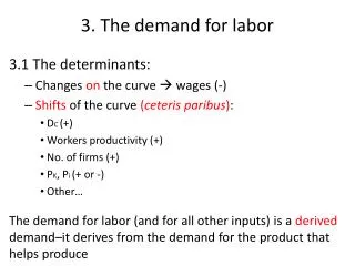
3. The Demand for Labor. Chapter Outline. Profit Maximization Marginal Income from an Additional Unit of Input Marginal Expense of an Added Input The Short-Run Demand for Labor When Both Product and Labor Markets Are Competitive A Critical Assumption: Declining MP L

E N D
3 The Demand for Labor
Chapter Outline • Profit Maximization • Marginal Income from an Additional Unit of Input • Marginal Expense of an Added Input • The Short-Run Demand for Labor When Both Product and Labor Markets Are Competitive • A Critical Assumption: Declining MPL • From Profit Maximization to Labor Demand • The Demand for Labor in Competitive Markets When Other Inputs Can Be Varied • Labor Demand in the Long Run • More than Two Inputs • Labor Demand When the Product Market is Competitive • Maximizing Monopoly Profits • Do Monopolies Pay Higher Wages? • Policy Application: The Labor Market Effects of Employer Payroll Taxes and Wage Subsidies • Who Bears the Burden of a Payroll Tax? • Employment Subsidies as a Device to Help the Poor • Appendix 3A: Graphical Derivation of a Firm’s Labor Demand Curve
3.1 Profit Maximization • For products price-taking and inputs price-taking firm, profit-maximizing decisions by a firm mainly involve the question of whether, and how, to increase or decrease output. • The search for profit improving possibilities means that small (“marginal”) changes must be made almost daily: • Major decisions to open a new plant or introduce a new product line are relatively rare, once made. • Must approach profit maximization incrementally through the trial-and-error • process of small changes. • Incrementally decide on its optimal level of output by: • – Q ↑ when MR > MC • – Q ↓when MR < MC, and that • – Q is profit maximizing or loss minimizing when MR = MC. • A firm can expand or contract output only by altering its use of inputs (capital and labor). • – Use more of an input if its MRP (additional income) > MEI (additional expense). • – Reduce the employment of an input if its MRP < MEI. • – No further changes in an input are desirable if its MRP = MEI.
3.1 Profit Maximization • Marginal Income from an Additional Unit of Input • We assume that labor (L) and capital (K) are needed to produce a given level of output (Q). That is: • Q = f (L, K) • Marginal Product • Marginal product of labor:MPL = ΔQ/ΔL|K constant (3.1) • Marginal product of capital:MPK = ΔQ/ΔK|L constant(3.2) • Marginal Revenue • Recall that: • In perfectly or purely competitive product market: MR = AR = P • In imperfectly or impurely competitive product market: MR < AR = P
3.1 Profit Maximization Marginal Revenue Product Marginal revenue product of L: MRPL = MPL . MR (3.3a) VMPL = MRPL = MPL . P (3.3b) Marginal revenue product of K: MRPK = MPK . MR VMPL = MRPK = MPK . P Marginal Expense of an Added Input • ∆L and/or ∆K will add to or subtract from the firm’s total costs • Marginal expense of labor (MEL) is the change in total labor cost for each additional unit of labor hired • If the labor market is competitive, each worker hired is paid the same wage (W) as all other workers, hence: MEL = W → horizontalsupply curve • If the capital market is competitive, each additional unit of capital will have the same rental cost (C), hence: MEK = C
3.2 The Short-Run Demand for Labor When Both Product and Labor Markets Are Competitive • In the short-run, the firm cannot vary its stock of capital, therefore, the production function takes the form: • This means the firm needs only to decide whether to alter its output level; how to increase or decrease output is not an issue, because only the employment of labor (L) can be adjusted – see Table 3.1
3.2 The Short-Run Demand for Labor When Both Product and Labor Markets Are Competitive • When both product and labor markets are competitive, it is assumed that: • All producers or sellers are price takers in the product market. • All employers of labor are wage takers in the labor market. • Analysis of a firm’s production and employment is in the short run where the firm cannot vary its capital stock. • With short production, only the employment of labor can be adjusted.
3.2 The Short-Run Demand for Labor When Both Product and Labor Markets Are Competitive A Critical Assumption: Declining MPL • Since K is constant in the short-run, adding extra unit of Lincreases output in each case – MPL is positive to some point. • Eventually, adding more L will produce progressively smaller increments of output – law of diminishing marginal returns. • This means that as employment expands, each additional worker has a progressively smaller share of the capital stock to work with.
3.2 The Short-Run Demand for Labor When Both Product and Labor Markets Are Competitive From Profit Maximization to Labor Demand • Profits are maximized only when employment is such that any further one-unit change in labor would have a marginal revenue product equal to marginal expense: MRPL = MEL (3.4) MPL . P = W (3.5) MPL = W/P (3.6)
3.2 The Short-Run Demand for Labor When Both Product and Labor Markets Are Competitive Labor Demand in Terms of Real Wages • Labor demand can be analyzed in terms of either real or money wages. • The negative slope of the labor demand curve indicates that each additional unit of labor employed produces a progressively smaller increment in output. • At any real wage determined by the market, the firm should employ labor up to the point at which MPL equals the real wage (W/P) – the firm’s demand for labor in the short-run is equivalent to the downward-sloping segment of its MPL schedule: • At E0 employment level: MPL = W/P → profit maximizing level of employment. • At E1 employment level: MPL > W/P → employment level E1 is less than E0; firm could increase profit by adding L. • At E2 employment level: MPL < W/P → employment level E2is greater than E0; firm could increase profit by decreasing L.
3.2 The Short-Run Demand for Labor When Both Product and Labor Markets Are Competitive Labor Demand in Terms of Money Wages • In some circumstances, labor demand curves are more readily conceptualized as downward-sloping functions of money wages. • MRPLdoes not decline because added workers are incompetent, it declines because capital stock is fixed, hence added workers have less capital or equipment to work with. • The fundamental point is: the labor demand curve in the short-run slopes downward because it is the MRPL curve, which slopes downward because of labor’s diminishing marginal product. • Since MRPL =W for a profit maximizer who takes wages as given, the MRPL curve and labor demand curve (MPL) must be the same. • The marginal product of an individual is not a function solely of his or her personal characteristics: • It depends on the number of similar employees hired by the firm and the firm’s capital stock.
3.2 The Short-Run Demand for Labor When Both Product and Labor Markets Are Competitive Market Demand Curves • A market demand curve(or schedule) is the summation of the labor demanded by all firms in a particular labor market at each level of the real wage • When real wage changes (falls or increases), the number of workers that existing firms want to employ changes (increases or falls) Objections to the Marginal Productivity Theory of Demand • Employers do not go around verbalizing MRPL – it is a theoretical concept, which assumes a degree of sophistication that most employers do not have • With fixed capital stock, it seems that adding labor would not add to output at all – but workers take their turns in using the fixed capital stock such that labor will generally have a marginal product greater than zero
3.3 The Demand for Labor in Competitive Markets When Other Inputs Can be Varied Labor Demand in the Long Run • In long-run, the firm’s ability to adjust other inputs such as capital will affect the demand for labor • To maximize profits in the long-run, the firm must adjust L and K such that each input’s MRP is equal to its ME MPL.P = W (a restatement of equation 3.5) (3.7a) MPK.P = C (the profit maximizing condition for K) (3.7b) Rearranging equations (3.7a) and (3.7b) yields: P = W/MPL (3.8a) P = C/MPK (3.8b) W/MPL = C/MPK (3.8c)
3.3 The Demand for Labor in Competitive Markets When Other Inputs Can be Varied • is the added cost or marginal cost (MC) of producing an added unit of output when using labor to generate the increase in output • is the marginal cost (MC) of producing an extra unit of output when using capital to generate the increase in output • To maximize profits, the firm must adjust its labor and capital inputs so that the marginal cost of producing an added unit of output using labor is equal to the marginal cost of producing an added unit of output using capital
3.3 The Demand for Labor in Competitive Markets When Other Inputs Can be Varied • Given = in equation (3.8c), if W increases: • Adjustment will have to be made to the use of labor (L). • The firm will have to cut back on the use of L, which will raise its MPL. • Each unit of capital (K) has less labor (L) working with it, therefore, MPK falls and the firm’s profit-maximizing level of level output will fall – scale effect. • Since > and if L↓ given an ↑W, the MPL↑ and the ↓MPKwill adjust to restore = . • The rise in W can also cause the firm to change its input mix by substituting capital for labor – substitution effect.
3.3 The Demand for Labor in Competitive Markets When Other Inputs Can be Varied More Than Two Inputs • Capital and labor are not the only inputs used in the production process. • Labor can be subdivided into many categories – by age, educational level, and occupation. • Other inputs in the production process include materials and energy. • For all other inputs, the equality of MC in using these inputs to produce an added unit of output as given by equation (3.8c) applies.
3.3 The Demand for Labor in Competitive Markets When Other Inputs Can be Varied If Inputs Are Substitute in Production • If two inputs are substitutes in production, and if an increase in the price of one input shifts the demand for another input to the left as in panel (a) of Figure 3.3, then the scale effect dominates the substitution effect – inputs are gross complements. • If the increase in the price of one input shifts the demand for the other input to the right as indicated in panel (b) of Figure 3.3, then the substitution effect dominates – inputs are gross substitutes. If Inputs Are Complements in Production • When two inputs must be used together in some proportion, they are considered to be perfect complements or complements in production – that is, no substitution effect, only scale effect.
Figure 3.3Effect of Increase in the Price of One Input (k) on Demand for Another Input (j), Where Inputs Are Substitutes in Production
3.4 Labor Demand When the Product Market Is Not Competitive • Monopoly producers are price-makers in the product market but wage-takers in the labor market. • They use MRPL = MEL to determine the profit-maximizing level of employment. Maximizing Monopoly Profits • To maximize monopoly profits, a monopolist will hire until: MRPL = MR.MPL = W (3.9) • Dividing both sides by P (recall that P > MR) yields: (3.10)
3.4 Labor Demand When the Product Market Is Not Competitive Do Monopolies Pay Higher Wages? • Economists suspect that product-market monopolies pay wages that are higher than what a competitive firms would pay and pass the costs along to consumers in the form of higher prices. • The ability to pay higher wages makes it possible for managers to hire people who might be more attractive or personable or have other characteristics managers find desirable.
3.5 Policy Application: The Labor Market Effects of Employer Payroll Taxes and Wage Subsidies • Governments finance certain social programs through taxes – payroll taxes – that require employers to remit payments based on their total payroll costs. Who Bears the Burden of a Payroll Tax? • Payroll taxes are used to finance government programs such as: • Unemployment insurance • Social Security retirement • Disability • Medicare/Medicaid • Let X be the fixed amount of tax per labor hour rather than a percentage of payroll.
3.5 Policy Application: The Labor Market Effects of Employer Payroll Taxes and Wage Subsidies Shifting the Demand Curve • Payroll taxes will shift the labor demand curve to the left. • Employers will decrease their employment of workers if their wage costs (wage bill) increase by the tax amount of X (that is, W+X ) due to payroll tax. • Employers will retain the same amount of workers as before the payroll tax was imposed if the entire tax burden is passed onto the workers, that is, workers’ wages fall by the tax amount of X (hence, W – X). • Employees bear a burden in the form of lower wage rates and lower employment levelswhen the government chooses to generate revenues through a payroll tax on employers.
Figure 3.4The Market Demand Curve and Effects of an Employer-Financed Payroll Tax
3.5 Policy Application: The Labor Market Effects of Employer Payroll Taxes and Wage Subsidies Effects of Labor Supply Curves • If the labor supply curve were vertical – meaning that lower or higher wages have no effect on labor supply – the entire amount of the tax will be shifted to workers in the form of a decrease in their wages by the amount of X(hence W – X). • The incidence of tax burden on employers and employees depends on the responsiveness (elasticities) of labor demand and labor supply to changes in wages. • If wages do not fall due to an employer payroll-tax increase, employment levels will, and employer labor costs will increase thus reducing the quantity of labor demanded.
3.5 Policy Application: The Labor Market Effects of Employer Payroll Taxes and Wage Subsidies Employment Subsidies as a Device to Help the Poor • Government subsidies of employers’ payroll could be in different forms: • Cash payments • Tax credit to employers – Target Job Tax Credit (TJTC), 1979-1995 • Generalor selective/targeted. • Let X be the fixed amount of subsidy that the government paid the employer per labor hour. • Subsidies shift the labor demand curve to the right, thus creating pressures to increase employment levels and the wages received by employees.
3A Graphical Derivation of a Firm’s Labor Demand Curve
The Production Function Q = f (L, K) Figure 3A.1: A Production Function
The Slope of the Isoquant • Along any isoquant, K can be decreased for much larger increase in L, but Q will remain unchanged • That is, labor could be substituted for capital to maintain a given level of production (ΔQ = 0): – ΔK.MPK + ΔL.MPL = 0 = – ΔK.MPK= ΔL.MPL or
Demand for Labor in the Short Run • Earlier in the Chapter, we assumed that capital is fixed in the short-run hence and that labor is hired • until labor’s MPL = W/P • Holding capital constant at Ka, the firm can produce: Q = 100 by employing La workers • Q = 150 by employing La’workers • Q = 200 by employing La” workers • The extra labor (La”– La’ ) required to produce 50 units of added output is greater than the extra labor (La’ – La) that produced the first 50-unit increment – see Figure 3A.2. • The assumptions that MPL declines as employment is increased and that firms hire until MPL = W/P are the bases for the assertion that a firm’s short-run demand curve for labor slopes downward.
Demand for Labor in the Long Run • Recall that a firm maximizes its profits by producing at a level of output (Q*) where MC = MR. • For a competitive firm, MR is equal to output/product price,that is, P = MR. • Conditions for Cost Minimization • How will the firm combine labor and capital to produce the Q*? • Profit maximization is possible if Q* is produced using the least expensive method. • Cost of producing Q* can be given by three isoexpenditure lines: • Line AA’ : 20K + 10L = 1,000 • Line BB’: 20K + 10L = 1,500 • Line DD’: 20K + 10L = 2,000
Figure 3A.3 Cost Minimization in the Production of Q* (Wage = $10 per Hour; Price of a Unit of Capital = $20)
The MRTS as defined in equation (3A.1) can be rewritten as: Rearranging, Slope of the isoexpenditure line is: . At the cost minimizing point: [a rearranged version of equation (3.8c)] Since MRTS is (see equation 3A.2) and equating this version of the MRTS to :
The Substitution Effect • Isoexpenditure line BB’ shows the cost minimizing point in producing Q* where the wage rate is $10 and the rental cost of capital is $20, which remained constant when the wage rate increased to $20 (doubled). • ↑W to $20 rotates the isoexpenditure line BB’ inward to BB” and it is no longer tangent to isoquant Q*, that is, Q* can no longer be produced for $1,500. • It is assumed that the least-cost expenditure to produce Q* increases to $2,250 and EE’ is the new isoexpenditure line. • The increased labor cost will induce the firm to substitute capital for labor – see point Z’ in Figure 3A.4. • The reduction in employment from LZ to LZ’is the substitution effect generated by the wage increase.
Figure 3A.4 Cost Minimization in the Production of Q*(Wage = $20 per Hour; Price of a Unit of Capital = $20)
The Scale Effect • Suppose that the profit-maximizing level of output falls from Q* to Q** and that all isoexpenditure lines have a new slope of 1 when W = $20 and C = $20 – see Figure 3A.5. • The cost-minimizing way to produce Q** is at Z” where the isoexpenditure line FF’ is tangent to the Q** isoquant. • The overall response in employment of labor due to the increase in the wage rate is the fall in labor usage from LZ to LZ”. • Recall that the decline from LZ to LZ’ is know as the substitution effect due to a wage change. • The scale effect is the reduction in employment from LZ’ to LZ” – reduction in the usage of both K (at KZ” – not shown) and L (at LZ”) because of the reduced scale of production.
Figure 3A.5 The Substitution and Scale Effects of a Wage Increase