Download

1 / 49
490 likes | 806 Views
Sequence Alignment. Outline. Global Alignment Scoring Matrices Local Alignment Alignment with Affine Gap Penalties. Section 1: Global Alignment. From LCS to Alignment: Change the Scoring.

E N D
Outline • Global Alignment • Scoring Matrices • Local Alignment • Alignment with Affine Gap Penalties
From LCS to Alignment: Change the Scoring • Recall: The Longest Common Subsequence (LCS) problem allows only insertions and deletions (no mismatches). • In the LCS Problem, we scored 1 for matches and 0 for indels, so our alignment score was simply equal to the total number of matches. • Let’s consider penalizing mismatches and indels instead.
From LCS to Alignment: Change the Scoring • Simplest scoring schema: For some positive numbers μ and σ: • Match Premium: +1 • Mismatch Penalty: –μ • Indel Penalty: –σ • Under these assumptions, the alignment score becomes as follows: Score = #matches – μ(#mismatches) – σ(#indels) • Our specific choice of µ and σ depends on how we wish to penalize mismatches and indels.
The Global Alignment Problem • Input : Strings v and w and a scoring schema • Output : An alignment with maximum score • We can use dynamic programming to solve the Global Alignment Problem: if vi = wj if vi ≠ wj m : mismatch penalty σ : indel penalty
Scoring Matrices • To further generalize the scoring of alignments, consider a (4+1) x (4+1) scoring matrixδ. • The purpose of the scoring matrix is to score one nucleotide against another, e.g. A matched to G may be “worse” than C matched to T. • The addition of 1 is to include the score for comparison of a gap character “-”. • This will simplify thealgorithm to the dynamicformula at right: Note: For amino acid sequence comparison, we need a (20 + 1) x (20 + 1) matrix.
Scoring Matrices: Example • Say we want to align AGTCA and CGTTGG with the following scoring matrix: AGTCA CGTTGG Score: –0.6 – 1 + 1 + 1 – 0.5 – 1.5 – 0.8 = –2.4 Sample Alignment:
Percent Sequence Identity • Percent Sequence Identity: The extent to which two nucleotide or amino acid sequences are invariant. • Example: A C C T G A G – A G A C G T G – G C A G mismatch indel 7/10 = 70% identical
How Do We Make a Scoring Matrix? • Scoring matrices are created based on biological evidence. • Alignments can be thought of as two sequences that differ due to mutations. • Some of these mutations have little effect on the protein’s function, therefore some penalties, δ(vi , wj), will be less harsh than others. • This explains why we would want to have a scoring matrix to begin with.
AKRANR KAAANK -1 + (-1) + (-2) + 5 + 7 + 3 = 11 Scoring Matrix: Positive Mismatches • Notice that although R and K are different amino acids, they have a positive mismatch score. • Why? They are both positively charged amino acids this mismatch will not greatly change the function of the protein.
AKRANR KAAANK -1 + (-1) + (-2) + 5 + 7 + 3 = 11 Scoring Matrix: Positive Mismatches • Notice that although R and K are different amino acids, they have a positive mismatch score. • Why? They are both positively charged amino acids this mismatch will not greatly change the function of the protein.
AKRANR KAAANK -1 + (-1) + (-2) + 5 + 7 + 3 = 11 Scoring Matrix: Positive Mismatches • Notice that although R and K are different amino acids, they have a positive mismatch score. • Why? They are both positively charged amino acids this mismatch will not greatly change the function of the protein.
Mismatches with Low Penalties • Amino acid changes that tend to preserve the physicochemical properties of the original residue: • Polar to Polar • Aspartate to Glutamate • Nonpolar to Nonpolar • Alanine to Valine • Similarly-behaving residues • Leucine to Isoleucine
Scoring Matrices: Amino Acid vs. DNA • Two commonly used amino acid substitution matrices: • PAM • BLOSUM • DNA substitution matrices: • DNA is less conserved than protein sequences • It is therefore less effective to compare coding regions at the nucleotide level • Furthermore, the particular scoring matrix is less important.
PAM • PAM: Stands for Point Accepted Mutation • 1 PAM = PAM1 = 1% average change of all amino acid positions. • Note: This doesn’t mean that after 100 PAMs of evolution, every residue will have changed: • Some residues may have mutated several times. • Some residues may have returned to their original state. • Some residues may not changed at all.
PAMX • PAMx = PAM1x (x iterations of PAM1) • Example: PAM250 = PAM1250 • PAM250 is a widely used scoring matrix: Ala Arg Asn Asp Cys Gln Glu Gly His Ile Leu Lys ... A R N D C Q E G H I L K ... Ala A 13 6 9 9 5 8 9 12 6 8 6 7 ... Arg R 3 17 4 3 2 5 3 2 6 3 2 9 Asn N 4 4 6 7 2 5 6 4 6 3 2 5 Asp D 5 4 8 11 1 7 10 5 6 3 2 5 Cys C 2 1 1 1 52 1 1 2 2 2 1 1 Gln Q 3 5 5 6 1 10 7 3 7 2 3 5 ... Trp W 0 2 0 0 0 0 0 0 1 0 1 0 Tyr Y 1 1 2 1 3 1 1 1 3 2 2 1 Val V 7 4 4 4 4 4 4 4 5 4 15 10
BLOSUM • BLOSUM: Stands for Blocks Substitution Matrix • Scores are derived from observations of the frequencies of substitutions in blocks of local alignments in related proteins. • BLOSUM62 was createdusing sequences sharingno more than 62% identity. • A sample of BLOSUM62is shown at right. http://www.uky.edu/Classes/BIO/520/BIO520WWW/blosum62.htm
Local Alignment: Why? • Two genes in different species may be similar over short conserved regions and dissimilar over remaining regions. • Example: Homeobox genes have a short region called the homeodomain that is highly conserved among species. • A global alignment would not find the homeodomain because it would try to align the entire sequence. • Therefore, we search for an alignment which has a positive score locally, meaning that an alignment on substrings of the given sequences has a positive score.
Local Alignment: Illustration Compute a “mini” Global Alignment to get Local Alignment Global alignment
Local vs. Global Alignment: Example • Global Alignment: • Local Alignment—better alignment to find conserved segment: --T—-CC-C-AGT—-TATGT-CAGGGGACACG—A-GCATGCAGA-GAC | || | || | | | ||| || | | | | |||| | AATTGCCGCC-GTCGT-T-TTCAG----CA-GTTATG—T-CAGAT--C tccCAGTTATGTCAGgggacacgagcatgcagagac |||||||||||| aattgccgccgtcgttttcagCAGTTATGTCAGatc
The Local Alignment Problem • Goal: Find the best local alignment between two strings. • Input : Strings v andw as well as a scoring matrix δ • Output : Alignment of substrings of v and w whose alignment score is maximum among all possible alignments of all possible substrings of v and w.
Local Alignment: How to Solve? • We have seen that the Global Alignment Problem tries to find the longest path between vertices (0,0) and (n,m) in the edit graph. • The Local Alignment Problem tries to find the longest path among paths between arbitrary vertices (i,j) and (i’, j’) in the edit graph.
Local Alignment: How to Solve? • We have seen that the Global Alignment Problem tries to find the longest path between vertices (0,0) and (n,m) in the edit graph. • The Local Alignment Problem tries to find the longest path among paths between arbitrary vertices (i,j) and (i’, j’) in the edit graph. • Key Point: In the edit graph with negatively-scored edges, Local Alignment may score higher than Global Alignment.
The Problem with This Setup • In the grid of size n x n there are ~n2 vertices (i,j)that may serve as a source. Local alignment Global alignment
The Problem with This Setup • In the grid of size n x n there are ~n2 vertices (i,j)that may serve as a source. • For each such vertex computing alignments from (i,j) to (i’,j’) takes O(n2) time.
The Problem with This Setup • In the grid of size n x n there are ~n2 vertices (i,j)that may serve as a source. • For each such vertex computing alignments from (i,j) to (i’,j’) takes O(n2) time.
The Problem with This Setup • In the grid of size n x n there are ~n2 vertices (i,j)that may serve as a source. • For each such vertex computing alignments from (i,j) to (i’,j’) takes O(n2) time.
The Problem with This Setup • In the grid of size n x n there are ~n2 vertices (i,j)that may serve as a source. • For each such vertex computing alignments from (i,j) to (i’,j’) takes O(n2) time.
The Problem with This Setup • In the grid of size n x n there are ~n2 vertices (i,j)that may serve as a source. • For each such vertex computing alignments from (i,j) to (i’,j’) takes O(n2) time.
The Problem with This Setup • In the grid of size n x n there are ~n2 vertices (i,j)that may serve as a source. • For each such vertex computing alignments from (i,j) to (i’,j’) takes O(n2) time. • This gives an overall runtime of O(n4), which is a bit too slow…can we do better?
Local Alignment Solution: Free Rides • The solution actually comes from adding vertices to the edit graph. • The dashed edges represent the“free rides” from (0, 0) to everyother node. • Each “free ride” is assignedan edge weight of 0. • If we start at (0, 0) instead of(i, j) and maximize the longestpath to (i’, j’), we will obtainthe local alignment. Yeah, a free ride!
Smith-Waterman Local Alignment Algorithm • The largest value of si,jover the whole edit graph is the score of the best local alignment. • The recurrence: • Notice that the 0 is the only difference between the global alignment recurrence…hence our new algorithm is O(n2)!
Scoring Indels: Naïve Approach • In our original scoring schema, we assigned a fixed penalty σto every indel: • -σ for 1 indel • -2σ for 2 consecutive indels • -3σ for 3 consecutive indels • Etc. • However…this schema may be too severe a penalty for a series of 100 consecutive indels.
Affine Gap Penalties • In nature, a series of k indels often come as a single event rather than a series of k single nucleotide events: • Example: More Likely Less Likely ATAG_GC AT_GTGC ATA__GC ATATTGC Normal scoring would give the same score for both alignments
Accounting for Gaps • Gap: Contiguous sequence of spaces in one of the rows of an alignment. • Affine Gap Penalty for a gap of length x is: -(ρ +σx) • ρ > 0 is the gap opening penalty: penalty for introducing a gap. • σ > 0 is the gap extension penalty: penalty for each indel in a gap. • ρ should be large relative to σ, since starting a gap should be penalized more than extending it.
Affine Gap Penalties • Gap penalties: • -ρ – σ when there is 1 indel, • -ρ– 2σ when there are 2 indels, • -ρ– 3σ when there are 3 indels, • -ρ –x·σ when there are x indels.
Affine Gap Penalties and the Edit Graph • To reflect affine gap penalties,we have to add “long”horizontal and vertical edgesto the edit graph. Each suchedge of length x should have weight
Affine Gap Penalties and the Edit Graph • To reflect affine gap penalties,we have to add “long”horizontal and vertical edgesto the edit graph. Each suchedge of length x should have weight • There are many such edges!
Affine Gap Penalties and the Edit Graph • To reflect affine gap penalties,we have to add “long”horizontal and vertical edgesto the edit graph. Each suchedge of length x should have weight • There are many such edges! • Adding them to the graphincreases the running time of alignment by a factor of n to O(n3).
Affine Gap Penalties and 3 Layer Manhattan Grid • The three recurrences for the scoring algorithm creates a 3-layered graph. • The main level extends matches and mismatches. • The lower level creates/extends gaps in sequence v. • The upper level creates/extends gaps in sequence w. • A jumping penalty is assigned to moving from the main level to either the upper level or the lower level (-ρ – σ). • There is a gap extension penalty for each continuation on a level other than the main level (- σ).
Visualizing Edit Graph: Manhattan in 3 Layers ρ δ δ σ δ ρ δ δ σ
The 3-leveled Manhattan Grid Gaps in w Matches/Mismatches Gaps in v