Download
1 / 16
160 likes | 174 Views
Cymbal Synthesis. Stefan Bilbao Music Edinburgh. Shell Models Finite Difference Schemes Computational Issues in Synthesis. Cymbal Modeling. Cymbals: an interesting synthesis problem: Simple PDE decription Regular geometry Highly nonlinear Time-domain methods are a very good match

E N D
Cymbal Synthesis Stefan BilbaoMusic Edinburgh • Shell Models • Finite Difference Schemes • Computational Issues in Synthesis
Cymbal Modeling Cymbals: an interesting synthesis problem: • Simple PDE decription • Regular geometry • Highly nonlinear Time-domain methods are a very good match (modal methods another possibility: ASA paper by Camier et al. on Tuesday)
Crashes Nonlinear effects are perceptually dominant: spontaneous generation of high frequencies (crash) A linear model is wholly insufficient!
A Shell Model Parameters: • Young’s modulus E • Poisson’s ratio n • Density r • Thickness h • Radius of curvature a • Size R Spherical shell model employed by, e.g., Thomas, Touze, Chaigne in recent work is a good rough approximation; Basic assumptions: shell is thin, shallow, uniform thickness and density + various other more technical hypotheses. r 0 Radial coordinate r Angular coordinate q Transverse displacement w(r,q, t) w(r,q, t) R h q a
A Nonlinear System System is an extension of that describing a thin flat, lossless, linear plate: Linear plate model: Nonlinearity: Airy stress function: Bracket operator: Shell curvature: Loss terms: Excitation:
Boundary and Center Conditions Free edge condition: Center conditions: Unconstrained: Clamped: Others possible: pivoting, with collision, perhaps loss
Difference Schemes in Polar Coordinates Polar cordinates a natural choice: Spacing hr in radial direction, hq in angular direction Total grid size: Approx. 2p/ hr hq points Operation count/time step will scale with this number of points… rhq hr
Bi-Laplacian operator in Polar Coordinates Key operation to approximate is the bi-Laplacian: DD A sparse operation… DD Needs to be specialized at: Grid points at or bordering the center, using center conditions: Grid points at or bordering the edge, using B.C.s: Also need approximations to the Laplacian, and to operators in bracket…
Implicit Schemes • One implicit family of schemes for the shell equations is the following: Free tuning parameter Explicit disc. of nonlinear terms; can stabilize by using implicit disc.! • Solution advanced as follows: 1. Determine Fn from known wn 2. Determine wn+1 from known Fn, wn 3. Update variables and repeat…
Implicit vs. Explicit The use of a good implicit scheme is essential, especially in the nonlinear case. Numerical “cutoff” Explicit a=0 Implications of low numerical cutoff: • Linear case: severe dispersion, mistuning of modes • Nonlinear case: inability of scheme to generate high-frequency energy! Energy “piles up” at cutoff…sounds terrible! Implicit a=0.2497 A problem, generally, for methods working over non-uniform grids…
Excitation • In a full physical model, need a model of the stick/mallet interaction • Simpler, in practice, to use an external forcing function • Here, g represents the spatial extent of the mallet, and h(t) the time history of the gesture
Effects of Curvature • The main effects of increased curvature are: • Decreased sense of a hum tone • Shifting upward of lowest frequencies, to give a brighter timbre… • Sound examples: for k=100, and for different values of the curvature parameter g, • In addition, computing time decreases with increased curvature…(fewer DOFs in audio range) g = 0 g = 40 g = 60 g = 100
Stability • A stabilitiy condition follows for the above scheme:
Implementation • Useful to reorder the grid functions w, F as vectors: DD • Update becomes a pair of linear systems to solve: • where are known (previously computed) vectors
Fast Linear System Solution Techniques: Structured Matrices • Various approaches to solving these systems: • Calculate inverses offline (a bad idea) • Use standard linear system solvers (Gauss-Seidel, SOR, CG, etc.) • Note: system matrices are very sparse, and possess a great deal of structure---which can be exploited: Circulant blocks (from periodicity in angular direction) Can employ DFTs to simplify structure: • Essentially a deconvolution operation in the angular direction • System is even more sparse much faster linear system solution • Only works in polar coordinates! (But can generalize to fast block-Toeplitz linear system solution in Cartesian coordinates)
Conclusions • Extensions: • More complex center conditions • Variable thickness • Generalized curvature • Lumped element connections (sizzles)