Download
1 / 30
310 likes | 486 Views
Eufar-ARSA meeting 2008. Synergy of radar, lidar and radiometer for observing ice clouds. Julien Delanoë & Robin Hogan University of Reading, UK. Clouds and remote sensing. Eufar-ARSA meeting 2008. Cloud radar 35GHz or 94GHz Measurements : reflectivity (Z in dBZ)

E N D
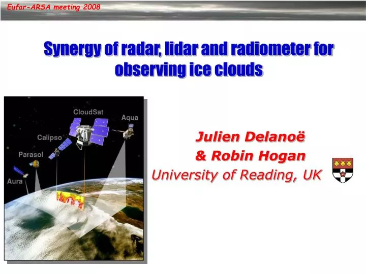
Eufar-ARSA meeting 2008 Synergy of radar, lidar and radiometer for observing ice clouds Julien Delanoë & Robin Hogan University of Reading, UK .
Clouds and remote sensing Eufar-ARSA meeting 2008 • Cloud radar 35GHz or 94GHz Measurements : reflectivity (Z in dBZ) Doppler velocity (Vd in m.s-1) Very sensitive to the size of the particles • Cloud lidar 532nm or 1064nm etc Measurements : attenuated backscatter (b in m-1 sr-1) Doppler velocity (Vd in m.s-1) Very sensitive to the concentration of the particles • Radiometers The measurement is integrated in the opposite of radar and lidar. It is very useful for radiativestudy of our atmosphere. • Radiance depends on vertical distribution of microphysical properties • Single channel: information on extinction near cloud top • Pair of channels: ice particle size information near cloud top => synergy of active and passive instruments Reflectivity radar [dBZ] Attenuated backscatter lidar [m-1 sr-1] Ground-base radar/lidar 1st April 2003 Palaiseau France (Frontal ice cloud)
Which platform for radar, lidar radiometers and what for ?Ground based, airborne, satellites ? Eufar-ARSA meeting 2008
Eufar-ARSA meeting 2008 Ground based Radar, lidar, radiometers + … continuous observation • CloudNET: Europe, 3 sites at the beginning: Cabauw / Chilbolton / Palaiseau • ARM(Atmospheric Radiation Measurement): World wide, several sites Ideally designed for local climatology and statistical validations of climate/forecast models and satellites. Airborne Radar-Lidar • For example RALI (RAdar LIdar) • Intensive observations periods • Ideally designed for detailed study case of clouds processes. • Demonstrator spatial, it can be use to validate Satellite measurement (flying under the trace of the Satellite, CloudSat/CALIPSO during AMMA sept 2006 etc) Satellites ! A-Train The CloudSat radar and the Calipso lidar were launched on 28th April 2006 (Cloud profiler lidar 532, 1064nm+ Infra Red Imager ; Cloud profiler radar 94GHz) They join Aqua, hosting the MODIS, CERES, AIRS and AMSU radiometers =>EarthCare (2013) • Need to combine all these observations to get an optimum estimate of global cloud properties
How to combine: Radar, lidar, radiometers Variational method Eufar-ARSA meeting 2008
Eufar-ARSA meeting 2008 An algorithm to combine radar, lidar, radiometers • Some limitations of existing radar/lidar ice retrieval schemes (Donovan et al. 2000, Tinel et al. 2005, Mitrescu et al. 2005) • Only work in regions of cloud detected by both radar and lidar • Noise in measurements results in noise in the retrieved variables • Other clouds in the profile are not included, e.g. liquid water clouds • Difficult to make use of other measurements, e.g. passive radiances • A “unified” variational scheme can solve all of these problems Delanoë and Hogan 2008, JGR (doi:10.1029/2007JD009000)
Formulation of variational scheme Ice visible extinction coefficient profile Attenuated lidar backscatter profile Ice normalized number conc. profile Radar reflectivity factor profile (on different grid) Extinction/backscatter ratio for ice Not yet Visible optical depth Liquid water path and number conc. for each liquid layer Infrared radiance Radiance difference Can be replaced by βmie and βray (HSRL) =>S is released Aerosol visible extinction coefficient profile Eufar-ARSA meeting 2008 • Observation vector (what we have) • State vector (which we want to retrieve) • Elements may be missing
Variational approach Forward Model: Convert first guess in observations Predicted observations Compare predicted observations and measurements, with an a-priori and measurement errors as a constraint Clever mathematics Iterative process Eufar-ARSA meeting 2008 Variational scheme : brief description We know the observations (instrument measurements) and we would like to know cloud properties : visible extinction, Ice water content, effective radius… Observations: whatever you want observation vector y First guess of clouds parameters, state vector x Direct Model, you don’t have to invert the measurements
Forward model a Z Eufar-ARSA meeting 2008 • Lookup tables: Derived from in-situ measurements We need a model to simulate observations from state vector To do that we use lookup tables and radar, lidar, radiative forward models. What kind of Lookup tables? for example we need a relationship between a and Z Unfortunately : this relationship is really scattered … So what can we do ?
Forward model N(D) Eufar-ARSA meeting 2008 The dimensional particle size distribution N(D) :PSD To simulate instrument measurements we need to know the particle concentration by unit of volume. If we know how are distributed ice particles in a sample volume, from the characteristic of one particle you can compute the characteristic of a volume => We can estimate the radar reflectivity for example : Radar Reflectivity [mm6.m-3] sbsc(D)backscatter coefficient (Mie,1908) Visible extinction [m-1] A(D) cross-section projected area N(D) is a key parameter !
N(D)=N0* F(D/D*) N0*: intercept parameter if exponential shape Z=f(a,N0*) N(D) N(D)/N0* a/N0* a Z D/D* Z/N0* Eufar-ARSA meeting 2008 Dimensional particle size distribution N(D) Very variable ! Different for each cloud • We use the normalization concept of particle size distribution (Delanoë et al. 2005): N(D)=N0*F(D/D*) where N0* is the normalization parameter and F the intrinsic shape (can be represented by a mathematical function) N(D) Scaled in Size by D* and in concentration by N0* Same for deriving re, IWC etc …
Radar forward model and a priori Example of relationship between N0*, a and T => Relationship more accurate than a N0*-T Eufar-ARSA meeting 2008 • A priori and first guess • First guess of a : constant value • N0* (Ice normalized number concentration) is computed from an a priori relationship between N0*, a and the temperature (derived from in situ measurements) • Radar forward model and lookup tables • We fix the mass-area-diameter relationships • Mie theory (95-GHz) for computing backscatter coefficient • The forward model predict Z from the extinction and N0* via : Z=f(a/N0*) • Effective radius via re=f(a/N0*) • Ice water content : IWC =f(a/N0*)
Lidar and radiance forward model Eufar-ARSA meeting 2008 • Lidar Multiple scattering New method (Hogan 2006) faster than Eloranta’s code usually used Attenuated backscatter profile : • From a profile and S (ratio a/b) and the Multiple scattering model (Hogan 2006) ba=f(a, Multiple Scattering contribution, S), with be=(1/S)a and • Infrared Radiances Radiance model uses the 2-stream source function method (Toon et al. (1989)) • Efficient yet sufficiently accurate method that includes scattering • Ice single-scatter properties from Anthony Baran’s aggregate model • Correlated-k-distribution for gaseous absorption (from David Donovan and Seiji Kato) • Radiative properties, asymetry factor, single-scatter albedo etc … as a function of a/NO* from lookup tables
Ground based application Eufar-ARSA meeting 2008
Ground based applications Eufar-ARSA meeting 2008 This kind of method is applied to ground based measurements, where radiometric measurements come from Meteo-Sat Second Generation, severi radiometer AMMA Campaign : ARM « Mobile Facility » Niamey Altitude:223 m Latitude:13.47 degree north Longitude:2.17 degree east Sample case : 22nd July 2006 • radar • lidar • Radiometer (msg), IR 8.7, 10.8, 12µm
Example from the AMF in Niamey Eufar-ARSA meeting 2008 Observed Radar Reflectivity 95-GHz Attenuated lidar backscatter return 523-nm Radar reflectivity Forward model Attenuated lidar backscatter Forward model Z radar b lidar
Results Radar+lidar only Large error where only one instrument detects the cloud Eufar-ARSA meeting 2008 Retrievals in regions where radar or lidar detects the cloud Retrieved visible extinction coefficient Retrieved effective radius Retrieval error in ln(extinction)
Results Radar, lidar, SEVERI radiances Cloud-top error is greatly reduced Retrieval error in ln(extinction) Eufar-ARSA meeting 2008 TOA radiances increase the optical depth and decrease particle size near cloud top Retrieved visible extinction coefficient Retrieved effective radius
Eufar-ARSA meeting 2008 Ice cloud properties from A-TRAINCloudSat-CALIPSO-AQUACase study
CALIPSO lidar Pacific Ocean 2006-9-22 Visible extinction Forward modelled lidar Ice water content CloudSat radar Effective radius Forward modelled radar • MODIS radiance 10.8um • Forward modelled radiance Eufar-ARSA meeting 2008
Eufar-ARSA meeting 2008 Ice cloud properties from A-TRAINCloudSat-CALIPSOStatistics/Model Comparison :one month data July 2006
Radar+lidar only log10(IWC) log10(IWC) Radar only Lidar only log10(IWC) log10(IWC) Eufar-ARSA meeting 2008 Frequency of occurrence of IWC vs temperature IWC increases with temperature: • but spread over 2 to 3 orders of magnitude at low temperatures • reach 5 orders of magnitude close to 0° C Advantage of the algorithm: Deep ice clouds: radar Thin ice clouds: lidar When radar and lidar work well together very good confidence in the retrievals • Obvious complementarity radar-lidar
Thanks to Richard Forbes (ECMWF) Alejandro Bodas-Salcedo (Met-Office) A-Train vs UK met-Office A-Train vs ECMWF A-Train vs ECMWF IWC cut-off @ 10-4 kg m-3 between 0°C & -20°C: explained by the parameterization of the ice-to-snow autoconversion rate. When ice water contents reach 10-4 kg m-3 => precipitating snow. Eufar-ARSA meeting 2008 Forecasts Vertical profiles were extracted from the model along the CloudSat-Calipso tracks at the closest time to the observations A-train data averaged to models grid Good trend but can’t capture variability lack of IWC @ T< -50°C => Models capture the trend of the IWC-T distribution (not the rest)
Conclusion Eufar-ARSA meeting 2008 Conclusion • New variational scheme, combining radar, lidar, radiometer and/or any other relevant measurement in order to retrieve cloud properties profiles Ongoing work: • Derive several lookup tables from different in-situ database • Retrieve properties of liquid-water layers, drizzle and aerosol • Incorporate microwave radiances for deep precipitating clouds • A-train data and validate using in-situ underflights • Quantify radiative errors in representation of different sorts of cloud
Supercooled water layers These pixels are not retrieved Can be bad detection Attenuated lidar backscatter from CALIPSO Radar Reflectivity from CloudSat We have developed a simple cloud phase identification algorithm Cloud seen by lidar Temperature model (ECMWF) => Ice / Liquid water Simple method : Exploit the different response of radar and lidar in presence of supercooled liquid water: -Very strong lidar signal -Very weak radar signal Within a 300m cloud layer Cloud seen by radar
Eufar-ARSA meeting 2008 2006290115910-02507 17th oct 2006 13:30 13:37 UTC Attenuated lidar backscatter from CALIPSO Radar Reflectivity from CloudSat Good agreement between IIR and MODIS
Eufar-ARSA meeting 2008 Ice cloud properties 2006290115910-02507 13:30 13:37 UTC No discontinuities Between radar lidar and radar&lidar
Supercooled layers Eufar-ARSA meeting 2008 Radiances and supercooled layers b CALIPSO Z Cloudsat Radiances MODIS 11mm Forward model 11mm Molecular +Simulate Liquid layer in the Radiance Model as Black body Optical depth Time [s]