Review of Probability and Statistics Concepts (Chapter 3:Modeling Process Quality)

1. Review of Probability and Statistics Concepts(Chapter 3:Modeling Process Quality)

2. Definition of Quality and Quality Improvement • Quality: Quality is inversely proportional to variability. • Quality improvement: The reduction of variability in processes and products.

3. What is Variability? • Unpredictability in a measurable (quantitative or qualitative) quantity. • Examples of quantities whose future values are unpredictable: • We need a concept/method to represent such unpredictable quantities.

4. Random Variable • Engineering definition - A quantity of interest whose exact value is unpredictable. • Notation

5. Characterizing Random Variables – Describing Variation • By “characterize” we mean methods to quantitatively describe variation • Utilize the characterization to aid decision making in an environment with unpredictability • Statistical inference • Prediction

6. Characterizing Random Variables – Describing Variation • IE Examples • Sizing a receiving area for customers • Process adjustments in response to process output measurements • Accepting a large lot of parts based on an inspection of a sample • … • Your examples

7. Characterizing Random Variables – Describing Variation Diagram

8. Characterizing Random Variables – Describing Variation • Start with data – no assumptions made • Graphical descriptions • Compute statistics

9. Characterizing Random Variables – Describing Variation • Basic graphical and numerical characterizations of data • Graphical • Histogram • Box Plot • Numerical (i.e., statistics) • Central tendency • Variability

10. Histogram • Graph of observed frequencies vs. value • Visual display of • Shape • Location or central tendency • Scatter or spread

11. Histogram • Decisions to make when constructing a histogram. • # of intervals ( ). • Minimum, Maximum (±∞ OK). • Can affect the visual impression.

12. Example

13. Creating Histograms • Manually • Excel • Statgraphics • Other software

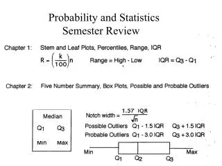
14. Box (and Whisker) Plot • Visual display of • Central tendency, Variability, Departure from symmetry, Outliers

15. Numerical Characterization: Values Computed from Data = Statistics • Measures of central tendency: • Sample Average (Sample mean) • Median (50th percentile) • Mode (Most frequent)

16. Numerical Characterization: Values Computed from Data = Statistics • Measures of variability reflected in the data • Sample variance • Sample standard deviation: • Sample Range:

17. Things to Notice • The sample average and sample variance are random variables • They are “quantities of interest whose exact value is unpredictable” • The sample variance is not affected by the location/magnitude of data, only by scatter about the sample average.

18. In-class Exercise Which route would you take? Why?

19. In-class Exercise

20. Now What? • The graphical and numerical values computed may meet your needs. • Examples • If the sample average of the time customers wait for service is less than x, then … • Travel time analysis for route choice

21. Now What? • Sometimes more in-depth analysis is required • Travel route example • If route 2 is selected what is the estimated probability that the travel time will be greater than x? • How certain am I that the true mean travel time for route 2 is less than the mean travel time for route 1? • What can be considered a maximum “typical” travel time for route 1? • IE examples

22. Now What? • Statistical inference – What conclusions can we make about a random variable and how certain are these conclusions. • Based on an assumed mathematical model for the behavior of the random variable

23. Characterizing Random Variables – Describing Variation • Describe the “behavior” of the random variable with mathematical models (functions) • What numerical quantities are used to characterize unpredictability? • The function used is a model • Justify/verify that it is a good model with data

24. Mathematical Models • You have seen a variety of mathematical models – exact outputs for given inputs • Thermodynamics, statics/dynamics, engineering economy

25. Mathematical Models of Variation • Mathematical models of unpredictable phenomena are different • If the model is accurate, it is accurate over many observations of the phenomena

26. Mathematical Models of Variation • Examples

27. Mathematical Models of Variation • IE examples

28. Mathematical Models of Variation • The uncertain behavior of a random variable is expressed in a mathematical function (this function is the model) • There are different types of functions utilized

29. Mathematical Models of Variation • How do we describe uncertain behavior? • i.e., What can be calculated from the mathematical functions describing uncertain behavior?

30. Mathematical Models of Variation • Two general types of random variables • Discrete – • Continuous – • Functions (terminology different than the text) • Probability/cumulative distribution functions • Density functions • Probability mass functions

31. Mathematical Models of Variation • Type of Random VariableFunctions from which probabilities can be found • Discrete - Probability Mass Function • Continuous - Probability Density Function Cumulative Distribution Function

32. Notation/Properties

33. Probability Mass Function for X 1 0.75 0.5 p(x) 0.25 0 0 1 2 X Discrete Random Variable • Discrete random variable – the possible values of a r.v. are “countable” . • E.g. Tossing two coins where the r.v. X is the number of heads

34. Continuous Random Variable • Continuous random variable can take on values in a continuous interval. • E.g. let r.v. X take values in interval [0, 2] Density Function

35. Questions • What are the two general types of random variables? • Give examples of both types. • What are the names of the functions used to characterize each type of random variable?

36. Probability/Cumulative Distribution Functions • Different than text! • Text uses “probability distribution function” = “prob. mass function”, and “prob. density function” • Probability/cumulative distribution function = Probability a random variable takes on a value less than or equal to some value x • Denoted

37. Probability/Cumulative Distribution Functions • For discrete random variables • F(x) is a summation of p(x) • For continuous random variables • F(x) is an integration of f(x)

38. Probability/Cumulative Distribution Functions • Examples

39. Example

41. Example

42. Mean/Expected Value • The Mean/Expected value of a random variable – often denoted as m • A measure of central tendency in the distribution

43. Variance • The variance of a random variable – often denoted s2 • A measure of scatter, spread or unpredictability in a distribution (in units2).

44. Question

45. Demonstration

46. Commonly Applied Discrete Distributions • Hypergeometric • Biniomial • Poisson • Pascal/Geometric

47. Commonly Applied Continuous Distributions • Normal • Lognormal • Exponential • Chi-Square • t-distribution • F-distribution • …

48. Demonstration

49. Normal Distribution • The most common probability model utilized in statistical inference procedures is the normal distribution

50. Normal Distribution • Notation • This is read: “X is normally distributed with mean m and standard deviation s.” • (Z represents a Standard Normal random variable)