Download
1 / 63
630 likes | 825 Views
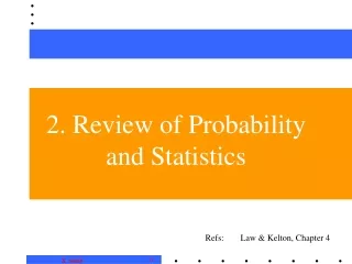
Ch.4 Review of Basic Probability and Statistics. 4.1 Introduction. Perform statistic analyses of the simulation output data. Design the simulation experiments. Probability and statistics. Model a probabilistic system. Generate random samples from the input distribution.

E N D
4.1 Introduction Perform statistic analyses of the simulation output data Design the simulation experiments Probability and statistics Model a probabilistic system Generate random samples from the input distribution Choose the input probabilistic distribution Validate the simulation model
4.2 Random variables and their properties • Experimentis a process whose outcome is not known with certainty. • Sample space(S) is the set of all possible outcome of an experiment. • Sample points are the outcomes themselves. • Random variable(X, Y, Z) is a function that assigns a real number to each point in the sample space S. • Values x, y, z
Examples • flipping a coin S={H, T} • tossing a die S={1,2,…,6} • flipping two coins S={(H,H), (H,T), (T,H), (T,T)} X: the number of heads that occurs • rolling a pair of dice S={(1,1), (1,2), …, (6,6)} X: the sum of the two dice
Distribution (cumulative) function : the probability associated with the event • Properties: • F(x) is nondecreasing [i.e., if ]. • .
Discrete random variable A random variable X is said to be discrete if it can take on at most a countable number of values. The probability that X takes on the value Then Probability mass function on I=[a,b]
p(x) 1 5/6 2/3 1/2 1/3 1/6 x 1 2 3 4 0 p(x) for the demand-size random variable X. Examples
F(x) 1 5/6 2/3 1/2 1/3 1/6 x 1 2 3 4 0 F(x) for the demand-size random variable X.
Continuous random variables A random variable is said to be continuous if there exists a nonnegative function f(x) such that for any set of real number B and f(x) is called the probability density function. for all
f(x) x Interpretation of the probability density function
F(x) f(x) 1 1 x x 0 1 0 1 f(x) for a uniform random variable on [0,1] F(x) for a uniform random variable on [0,1] where
f(x) 0 x Exponential random variable F(x) 1 0 x F(x) for an exponential random variable with mean f(x) for an exponential random variable with mean
Joint probability mass function If X and Y are discrete random variables, then let for all x, y where p(x,y) is called the joint probability mass function of X and Y. X and Y are independent if for all x, y where arethe(marginal) probability mass functions of X and Y.
Example 4.9 Suppose that X and Y are jointly discrete random variables with Then for x=1,2 for y=2,3,4 Since For all x, y, the random variables X and Y are independent.
Joint probability density function The random variables X and Y are jointly continuous if there exists a nonnegative function f(x,y), such that for all sets of real numbers A and B, X and Y are independent if for all x and y where are the (marginal) probability density functions of X and Y, respectively.
Example 4.11 Suppose that X and Y are jointly continuous random variables with Then for for Since X and Y are not independent.
Mean or expected value The mean is one measure of central tendency in the sense that it is the center of gravity
Examples 4.12-4.13 For the demand-size random variable, the mean is given by For the uniform random variable, the mean is given by
Properties of means 1. 2. Even if the ‘s are dependent.
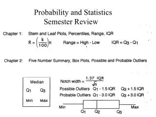
area=0.5 x Median The median of the random variable is defined to be the smallest value of x such that The median for a continuous random variable
Example 4.14 1. Consider a discrete random variable X that takes on each of the values, 1, 2, 3, 4, and 5 with probability 0.2. Clearly, the mean And the median of X are 3. 2. Now consider random variable Y that takes on each of the values, 1, 2, 3, 4, and 100 with probability 0.2. The mean and the median of X are 22 and 3, respectively. Note that the median is insensitive to this change in the distribution. The median may be a better measure of central tendency than the mean.
Variance For the demand-size random variable, For the uniform random variable on [0,1],
small large Density functions for continuous random variables with large and small variances.
Properties of the variance 1. 2. 3. if the ‘s are independent (or uncorrelated).
Standard deviation The probability that is between and is 0.95.
Covariance The covariance between the random variables and is a measure of their dependence. if i=j,
Example 4.17 For the jointly continuous random variables X and Y in Example 4.11
If and are independent random variables and are uncorrelated. Generally, the converse is not true.
Correlated If , then and are said to be positively correlated. and tend to occur together and tend to occur together If , then and are said to be negatively correlated. and tend to occur together and tend to occur together
Correlation If is close to +1, then and are highly positively correlated. If is close to -1, then and are highly negatively correlated. For the random variable in Example 4.11
4.3 Simulation output data and stochastic processes • Stochastic process is a collection of "similar" random variables • ordered over time, which are all defined on a common • sample space. State space is the set of all possible values that these random variables can take on. Discrete-time stochastic process: Continuous-time stochastic process:
Example 4.19 M/M/1 queue with IID interarrival times IID service times FIFO service Define the discrete-time stochastic process of delays in queue are positively correlated. and simulation input random variables output stochastic process The state space: the set of nonnegative real numbers
Example 4.20 For the queueing system of Example 4.19, Let be the number of customers in the queue at time t . Then is a continuous-time stochastic process with state space
Covariance-stationary Assumptions about the stochastic process are necessary to draw inferences in practice. is said to be A discrete-time stochastic process covariance-stationary, if and is independent of i for
Covariance-stationary process For a covariance-stationary process, the mean and variance are stationary over time, and the covariance between two observations and depends only on the separation j and not actual time valuei and i+j. We denote the covariance and correlation between and by and respectively, where
Example 4.22 Consider the output process for a covariance-stationary M/M/1 queue with .
Warmup period In general, output processes for queueing systems are positively correlated. If is a stochastic process beginning at time 0 in a simulation, then it is quite likely not to be covariance-stationary. However, for some simulation will be approximately covariance-stationary if k is large enough, where k is the length of the warmup period.
4.4 Estimation of means, variance, and correlations Suppose are IID random variables with finite population mean and finite population variance Unbiased estimators: Sample mean Sample variance
How close is to to construct a confidence interval Unbiased estimator
Density function for Density function for n large n small Distributions of for small and large n.
Estimate the variance of the sample mean . ´s are uncorrelated ´s are independent However, the simulation output data are almost always correlated. are from a covariance-stationary stochastic process, Then, is an unbiased estimator of , however, is no longer an unbiased estimator of . Since
However, simulation output data are always correlated. Since (1) For a covariance-stationary process: (2)
If one estimates from (correct in the IID case) • there are two errors: • the bias in as an estimator of . • the negligence of the correlation terms in Eq. (2). Solution: combine Eq. (1) and Eq. (2) (3) If , then and .
Example 4.24 from the process of delays for a covariance-stationary M/M/1 queue with . Eq.(1) and (3) Thus, is a gross underestimate of , and we are likely to be overly optimistic about the closeness of to
Estimate . In general "good" estimates of the 's will be difficult to obtain unless n is very large and j is small relative to n.