Review of Probability and Statistics

1. Review of Probability and Statistics Yen-Jen Oyang Department of Computer Science and Information Engineering National Taiwan University

2. Random Variable • A random variable X is a function that maps the outcomes of an experiment to real numbers. • That is X: S --> R, where S is a set of outcomes and R is the set of real numbers.

3. An Example of Random Variable • If we toss a coin one time, then there are two possible outcomes, namely “head up” and “tail up”. • We can define a random variable X that maps “head up” to 1 and “tail up” to 0. • We also can define a random variable Y that maps “head up” to 0 and “tail up” to 1.

4. Another Example of Random Variables • If we randomly pick up a bridge card, then we can define a random variable W that corresponds to the number on the card. • Also, we can define a random variable Z that corresponds to the color of the card. For example, Z = 1 if the card is a spade or club, and Z = 0 if the card is a heart or diamond.

5. Example of Continuous Random Variable • If we randomly pick up a real number between 0 and 1, then we define a continuous uniform random variable V with Prob(V  t) = t, for any real number 0 t 1

6. Probability Distribution Function • For a random variable X, we define its probability distribution function F as

7. Properties of a Probability Distribution Function • 1. • 2. • 3. , if w t. • Any function that satisfies these conditions above can be a distribution function.

8. Discrete/Continuous Random Variable • Given a random variable X, let S denote the set of possible outcomes of X. • If S is a finite or countable infinite set, then X is said to be a discrete random variable.

9. Countable Infinite • A set is said to be countable infinite, if it contains infinite number of elements and there exists a one-to-one mapping between each element of the set and the positive integers.

10. Examples of Countable / Uncountable Infinite • The set of integer numbers is countable. • The set of fractional numbers is countable. • The set of real numbers is uncountable.

11. Mapping of Integer Numbers to Positive Integer Numbers • 0 1 –1 2 –2 3 –3 …… • 0 1 2 3 4 5 6 ……

12. Mapping of Fractional Numbers to Positive Integer Numbers

13. Example of Discrete Random Variables • A Bernoulli random variable has only two outcomes, success and failure, with probabilities p and 1-p, respectively. • If we conduct a Bernoulli experiment n times and count the times of success, then we get a binomial random variable with parameters n, p and

14. Probability Mass/Density Function • The probability mass/density function of a random variable X is defined to be • , for discrete random variables • , for continuous random variables

15. Expected Value of a Random Variable • For discrete random variables: • For continuous random variables: •  is a widely used symbol for expected value.

16. Example of the Expected Value of a Random Variable • Assume that the probability of getting “head up” by tossing a coin is 0.7. If we toss the coin two times and define X to be the number of times that “head up” appears, then there are 4 possible outcomes, (0,0), (0,1), (1,0), and (1,1), in the outcome space of X.

17. ~Continued • Random Variable X has the following probability mass function: • P(0) = 0.3 * 0.3 = 0.09; • P(1) = 0.3 * 0.7 + 0.7 * 0.3 = 0.42; • P(2) = 0.7 * 0.7 = 0.49. • The expected value of X is equal to 0*0.09+1*0.42+2*0.49 = 1.4

18. Variance of Random Variables • The variance of a random variable is defined to be • For discrete random variables: • For continuous random variables:

19. Standard Deviation • The standard deviation of a random variable is the square root of its variance. •  is a widely used symbol for standard deviation.

20. Function of Random Variables • Let X be a random variable and G be a function. Then, random variable Y = G(X) maps an outcome v in the outcome set of X to value G(X(v)). • With respect to the probability distribution functions, if G(X) is one-to-one mapping, then

21. Example of Functions of Random Variables • If we toss a coin two times and let X correspond to the number of times that “head up” appears. Let Y=X2. Then, • Y((0,0)) --> 0; • Y((0,1)) --> 1; • Y((1,0)) --> 1; • Y((1,1)) --> 4;

22. Functions of Multiple Random Variables • Let X and Y be two random variables defined on the same outcome set and G() be a function with two parameters. Then, Z = G(X,Y) is a random variable defined on the same outcome set and maps outcome v to G(X(v),Y(v)).

23. ~Continued • For two random variables X1 and X2 defined on different two outcome sets S1 and S2, we can define a new outcome set by taking the product of S1 X S2 and redefine X and Y on the new outcome set. Then, we can create functions for X1 and X2. • For example, assume that we toss a $10 one time and later a $5 coins one time. Let X1 correspond to whether the $10 coin has a “head up” and X2 correspond to whether the $5 coin has a “head up”, respectively. Then, we can define a new outcome set for X1 and X2.

24. Jointly Distributed Random Variables • Let X and Y be two random variables defined on the same outcome space. The joint distribution function Fx,y of X and Y is defined as follows: • FX,Y(r,s) = Prob(X  r, Ys) • Furthermore,

25. Independent Discrete Random Variables • Two random variables X and Y defined on the same outcome space are said to be independent if and only if

26. Similarly, for two discrete random variable X, Y that are independent, we have PXY(r,s) = PX(r)  PY(s).

27. Example 1 of Independent Random Variables • Assume that we toss a coin two times. Let random variable X correspond to the outcome of the first tossing and Y correspond to the outcome of the second tossing. Then, X and Y are two independent random variables.

28. Example 2 of Independent Random Variables • Assume that we randomly pick up a bridge card. Let random variable X correspond to the color of the card and Y correspond to the number or figure on the card. Then, X and Y are independent.

29. Example of Positively/Negatively Correlated Random Variables • In the Bridge card example, let X correspond to whether the color of the card is black, Y correspond to whether the card is a club card, Z correspond to whether the card is a diamond card. Then, X and Y are positively correlated but X and Z are negatively correlated.

30. Mutually Independent and Jointly Indepentdent • Three random variables may be pairwisely independent but not jointly independently. • Let X, Y be the random variables corresponding to two independent trials of a Bernoulli experiment with p = 0.5. Let Z=XY. Then, X,Y and Z are pairwisely independent but not jointly independent.

31. Prob(X=0, Z=0) =Prob(X=0, Y=0) = 0.25 Prob(X=0)Prob(Z=0) = 0.25 • However, Prob(X=0, Y=0, Z=1) = 0 Prob(X=0)Prob(Y=0)Prob(Z=1) = 0.125

32. Addition and Scaling of Random Variables • Let X and Y be two random variables. Then, • E[X+Y] = E[X] + E[Y]. • E[cX] = cE[X]. • Var[cX] = c2Var[X].

34. Important Observations Regarding Two Independent Random Variables • Var[X+Y] = Var[X] + Var[Y], • i.e. E[XY] = E[X]E[Y] Proof:

35. Characteristics of Binomial Random Variables • A Binomial random variable X with parameters n, p has the following characteristics:

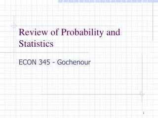
36. The Normal Distribution • A continuous random variable is said to have a normal distribution, if its probability density function is where t, R and  > 0. • A random variable with normal distribution is denoted by N(, 2)

38. Characteristics of Random Variables with Normal Distribution

42. The Standard Normal Distribution • A normal distribution N(,2) with  = 0 and  = 1 is said to be the standard normal distribution. • The p.d.f. of N( 0 , 1) is • A convention is using (x) to denote

43. Transformation of Random Variables with Normal Distribution

44. The Table of the Standard Normal Distribution

45. X 0.00 0.01 0.02 0.03 0.04 0.05 0.06 0.07 0.08 0.09 0.0 0.00000 0.00399 0.00798 0.01197 0.01595 0.01994 0.02392 0.02790 0.03188 0.03586 0.1 0.03983 0.04380 0.04776 0.05172 0.05567 0.05962 0.06356 0.06749 0.07142 0.07535 0.2 0.07926 0.08317 0.08706 0.09095 0.09483 0.09871 0.10257 0.10642 0.11026 0.11409 0.3 0.11791 0.12172 0.12552 0.12930 0.13307 0.13683 0.14058 0.14431 0.14803 0.15173 0.4 0.15542 0.15910 0.16276 0.16640 0.17003 0.17364 0.17724 0.18082 0.18439 0.18793 0.5 0.19146 0.19497 0.19847 0.20194 0.20540 0.20884 0.21226 0.21566 0.21904 0.22240 0.6 0.22575 0.22907 0.23237 0.23565 0.23891 0.24215 0.24537 0.24857 0.25175 0.25490 0.7 0.25804 0.26115 0.26424 0.26730 0.27035 0.27337 0.27637 0.27935 0.28230 0.28524 0.8 0.28814 0.29103 0.29389 0.29673 0.29955 0.30234 0.30511 0.30785 0.31057 0.31327 0.9 0.31594 0.31859 0.32121 0.32381 0.32639 0.32894 0.33147 0.33398 0.33646 0.33891 1.0 0.34134 0.34375 0.34614 0.34849 0.35083 0.35314 0.35543 0.35769 0.35993 0.36214 1.1 0.36433 0.36650 0.36864 0.37076 0.37286 0.37493 0.37698 0.37900 0.38100 0.38298 1.2 0.38493 0.38686 0.38877 0.39065 0.39251 0.39435 0.39617 0.39796 0.39973 0.40147 1.3 0.40320 0.40490 0.40658 0.40824 0.40988 0.41149 0.41308 0.41466 0.41621 0.41774 1.4 0.41924 0.42073 0.42220 0.42364 0.42507 0.42647 0.42785 0.42922 0.43056 0.43189 1.5 0.43319 0.43448 0.43574 0.43699 0.43822 0.43943 0.44062 0.44179 0.44295 0.44408 1.6 0.44520 0.44630 0.44738 0.44845 0.44950 0.45053 0.45154 0.45254 0.45352 0.45449 ~Continued

46. The Central Limit Theorem • Let X be a random variable with expected value u and standard variation . If we conduct the experiment n times and let • Then, the distribution function of approaches that of the standard normal distribution when n is sufficiently large.

47. A Formal Representation of the Central Limit Theorem

48. Approximation of the Binomial Distribution by the Standard Normal Distribution • Let X be a binomial random variable with n, p. Then, the distribution of can be approximated by the standard normal distribution. where () is the distribution function of the standard normal distribution.

49. The Chi-Squared Distribution • Let X be a random variable with the standard normal distribution. • Then, Z = X2has the so-called chi-square distribution with degree of freedom =1, and is denoted by 12.

50.  0.10 0.05 0.025 0.01 0.001 1 2.706 3.841 5.024 6.635 10.828 2 4.605 5.991 7.378 9.210 13.816 3 6.251 7.815 9.348 11.345 16.266 4 7.779 9.488 11.143 13.277 18.467 5 9.236 11.070 12.833 15.086 20.515 Critical Values of the Chi-Square Distribution