Download
1 / 28
280 likes | 430 Views
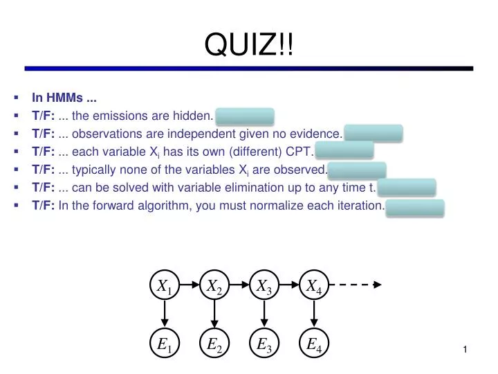
QUIZ!!. In HMMs ... T/F: ... the emissions are hidden. FALSE T/F: ... observations are independent given no evidence. FALSE T/F: ... e ach variable X i has its own (different) CPT. FALSE T/F: ... t ypically none of the variables X i are observed. TRUE

E N D
QUIZ!! • In HMMs ... • T/F: ... the emissions are hidden. FALSE • T/F: ... observations are independent given no evidence. FALSE • T/F: ... each variable Xi has its own (different) CPT. FALSE • T/F: ... typically none of the variables Xiare observed. TRUE • T/F: ... can be solved with variable elimination up to any time t. TRUE • T/F:In the forward algorithm, you must normalize each iteration. FALSE X1 X2 X3 X4 E1 E2 E3 E4
CSE 511a: Artificial IntelligenceSpring 2013 Lecture 20: HMMs Particle Filters 04/15/2012 Robert Pless via KilianQ. Weinberger w/ slides from Dan Klein – UC Berkeley
Announcements • Project 4 is up! • Due in one week!! • Contest Coming Soon
Recap: Reasoning Over Time • Stationary Markov models • Hidden Markov models 0.3 0.7 X1 X2 X3 X4 rain sun 0.7 0.3 X1 X2 X3 X4 X5 E1 E2 E3 E4 E5
Just like Variable Elimination X1 X2 X3 X4 e1 ¬e2 e3 e4 Emission probability: evidence
Just like Variable Elimination X1,e1 X2 X3 X4 ¬e2 e3 e4 Transition probability:
Just like Variable Elimination Marginalize out X1... X1,X2,e1 X3 X4 ¬e2 e3 e4
Just like Variable Elimination X2,e1 X3 X4 ¬e2 e3 e4 Emission probability:
Just like Variable Elimination X2,e1, ¬e2 X3 X4 e3 e4
The Forward Algorithm • We are given evidence at each time and want to know • We can derive the following updates We can normalize as we go if we want to have P(x|e) at each time step, or just once at the end…
X1 X2 X2 E2 Online Belief Updates • Every time step, we start with current P(X | evidence) • We update for time: • We update for evidence: • The forward algorithm does both at once (and doesn’t normalize) • Problem: space is |X| and time is |X|2 per time step
Best Explanation Queries • Query: most likely seq: X1 X2 X3 X4 X5 E1 E2 E3 E4 E5
State Path Trellis • State trellis: graph of states and transitions over time • Each arc represents some transition • Each arc has weight • Each path is a sequence of states • The product of weights on a path is the seq’s probability • Can think of the Forward algorithm as computing sums of all paths in this graph sun sun sun sun rain rain rain rain
Viterbi Algorithm sun sun sun sun rain rain rain rain
0.0 0.1 0.0 0.0 0.0 0.2 0.0 0.2 0.5 Particle Filtering • Sometimes |X| is too big to use exact inference • |X| may be too big to even store B(X) • E.g. X is continuous • |X|2 may be too big to do updates • Solution: approximate inference • Track samples of X, not all values • Samples are called particles • Time per step is linear in the number of samples • But: number needed may be large • In memory: list of particles, not states • This is how robot localization works in practice
Representation: Particles • Our representation of P(X) is now a list of N particles (samples) • Generally, N << |X| • Storing map from X to counts would defeat the point • P(x) approximated by number of particles with value x • So, many x will have P(x) = 0! • More particles, more accuracy • For now, all particles have a weight of 1 Particles: (3,3) (2,3) (3,3) (3,2) (3,3) (3,2) (2,1) (3,3) (3,3) (2,1)
Particle Filtering: Elapse Time • Each particle is moved by sampling its next position from the transition model • This is like prior sampling – samples’ frequencies reflect the transition probs • This world is a pacman world with default clockwise motions, so here, most samples move clockwise, but some move in another direction or stay in place • This captures the passage of time • If we have enough samples, close to the exact values before and after (consistent)
Particle Filtering: Observe • Slightly trickier: • Don’t do rejection sampling (why not?) • We don’t sample the observation, we fix it • This is similar to likelihood weighting, so we downweight our samples based on the evidence • Note that, as before, the probabilities don’t sum to one, since most have been downweighted (in fact they sum to an approximation of P(e))
Particle Filtering: Resample Old Particles: (3,3) w=0.1 (2,1) w=0.9 (2,1) w=0.9 (3,1) w=0.4 (3,2) w=0.3 (2,2) w=0.4 (1,1) w=0.4 (3,1) w=0.4 (2,1) w=0.9 (3,2) w=0.3 • Rather than tracking weighted samples, we resample • N times, we choose from our weighted sample distribution (i.e. draw with replacement) • This is equivalent to renormalizing the distribution • Now the update is complete for this time step, continue with the next one New Particles: (2,1) w=1 (2,1) w=1 (2,1) w=1 (3,2) w=1 (2,2) w=1 (2,1) w=1 (1,1) w=1 (3,1) w=1 (2,1) w=1 (1,1) w=1
Robot Localization • In robot localization: • We know the map, but not the robot’s position • Observations may be vectors of range finder readings • State space and readings are typically continuous (works basically like a very fine grid) and so we cannot store B(X) • Particle filtering is a main technique • [Demos,Fox]
Dynamic Bayes Nets (DBNs) • We want to track multiple variables over time, using multiple sources of evidence • Idea: Repeat a fixed Bayes net structure at each time • Variables from time t can condition on those from t-1 • Discrete valued dynamic Bayes nets are also HMMs t =1 t =2 t =3 G1a G2a G3a G1b G2b G3b E1a E1b E2a E2b E3a E3b
Exact Inference in DBNs • Variable elimination applies to dynamic Bayes nets • Procedure: “unroll” the network for T time steps, then eliminate variables until P(XT|e1:T) is computed • Online belief updates: Eliminate all variables from the previous time step; store factors for current time only t =3 t =1 t =2 G3a G1a G2a G3b G3b G1b G2b E3a E3b E1a E1b E2a E2b
DBN Particle Filters • A particle is a complete sample for a time step • Initialize: Generate prior samples for the t=1 Bayes net • Example particle: G1a = (3,3) G1b = (5,3) • Elapse time: Sample a successor for each particle • Example successor: G2a = (2,3) G2b = (6,3) • Observe: Weight each entire sample by the likelihood of the evidence conditioned on the sample • Likelihood: P(E1a |G1a ) * P(E1b |G1b ) • Resample: Select prior samples (tuples of values) in proportion to their likelihood
SLAM • SLAM = Simultaneous Localization And Mapping • We do not know the map or our location • Our belief state is over maps and positions! • Main techniques: Kalman filtering (Gaussian HMMs) and particle methods DP-SLAM, Ron Parr
Summary Filtering • Push Belief through time • Incorporate observations • Inference: • Forward Algorithm (/ Variable Elimination) • Particle Filter (/ Sampling) • Algorithms: • Forward Algorithm (Belief given evidence) • Viterbi Algorithm (Most likely sequence)