Download
1 / 57
570 likes | 744 Views
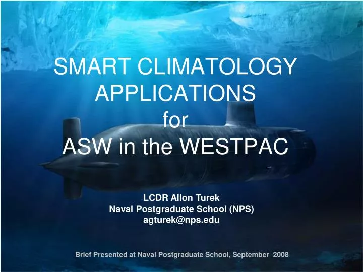
SMART CLIMATOLOGY APPLICATIONS for ASW in the WESTPAC. LCDR Allon Turek Naval Postgraduate School (NPS) agturek@nps.edu. Brief Presented at Naval Postgraduate School, September 2008. Overview. Purpose of this study Data sets used Methods Results Future research and development

E N D
SMART CLIMATOLOGY APPLICATIONS for ASW in the WESTPAC LCDR Allon Turek Naval Postgraduate School (NPS) agturek@nps.edu Brief Presented at Naval Postgraduate School, September 2008
Overview • Purpose of this study • Data sets used • Methods • Results • Future research and development • Recommendations
Purpose • Determine if the NPS Smart Climatology Process can be utilized to improve ASW support in the WESTPAC • Determine if state of the science ocean data sets offer an advantage over existing Navy data sets • Provide recommendations
Data Atmospheric Data National Center of Environmental Prediction (NCEP) Re-analysis • Daily and Monthly Values for 1948 - present. • Long term monthly means 1968 - 1996. • Simple Ocean Data Assimilation (SODA) • Global 0.5 x 0.5 deg resolution (1958-2001) • 40 depth levels (5m – 5374m) • Generalized Digital Environmental Model (GDEM) • Global 0.25 x 0.25 deg resolution (1900-1995) • 78 depth levels (0m – 6600m) Ocean Data
Methods • Application of NPS Smart Climatology Process • Time series analysis • Conditional climatology selection • Analysis of anomalies • Comparison of data sets • Extraction of T/S and sound speed profiles • Analysis of profile significance in PC-IMAT
Application of Smart Climatology Immediate desire for longer lead time and improved accuracy in range prediction Greater accuracy and lead time mean improved planning/increased PD Acquire SODA and GDEM datasets Examine years of highest and lowest winds for a given area Use climate analysis to choose subsets of database that are likely to be predictive of environment Predicted environment Compare predicted environment to expected physical processes (i.e. upwelling, downwelling, mass transport, mixing, etc…)
Smart Climatology vs. Traditional Climatology Smart climatology acknowledges climate oscillation signals such as (1) El Nino and La Nina, and studies how climate indices such as (2) the multivariate ENSO index can be used to help predict future environmental conditions through methods such as time series analysis, composites, correlations , and teleconnections. Traditional long term mean (LTM) climatology, simply compiles data and uses it to create (3) a mean value that may not be representative of the normal variability observed in the environment 1 2 3 (LTM)
SST Using Smart Climatology Time Series of Monthly Mean SST for October Upward Trend Mean of 10 strongest LaNinas 27.6° ( Smart climatology) 26.8° LTM ( traditional climatology) From the two values of SST it is clear that a smart climatology approach can give results that more closely represent increased SST values seen during a La Nina event. (Pre-satellite era data) Figure created at the NOAA/ESRL Physical Sciences Division, Boulder Colorado Web site at http://www.cdc.noaa.gov/Timeseries/
Meridional Wind Speed Time Series of Monthly Mean Meridional Wind Speed for October Mean of 5 weakest wind years -2.96 m/s ( smart climatology) LTM -4.54 m/s ( traditional climatology) Increasing Trend Mean of 5 strongest wind years -6.81 m/s ( smart climatology) Other conditional climatologies such as high and low wind composites are also capable of producing more realistic characterizations of the actual or expected environment than the LTM (Pre-satellite era data) Figure created at the NOAA/ESRL Physical Sciences Division, Boulder Colorado Web site at http://www.cdc.noaa.gov/Timeseries/
Conditional Climatology Selection • Focused on identifying atmospheric or climatological factors that: • Have a predictable affect on the ocean environment • Occur regularly • That are well researched and documented • This led to choosing high vs. low wind years • Choose a month or season with above average ocean variability • Transition between summer and winter monsoon provides large variability in ocean and atmosphere • This led to choosing the month of October
LTM Surface Winds Figure created using data from NOAA/ESRL Physical Sciences Division, Boulder Colorado Web site at http://www.cdc.noaa.gov/Composites/
Comparison of SODA and GDEM LTM Sea Surface Temps SODA (LTM) GDEM (LTM) The bull’s eye pattern seen in GDEM SSTs is an artifact of the GDEM interpolation scheme and is not representative of small scale ocean variability Figure created using data from SODA ocean reanalysis. Department of Atmospheric and Oceanic Science, University of Maryland. http://www.atmos.umd.edu/~ocean/data.html
Comparison of SODA and GDEM LTM Sea Surface Heights SODA (LTM) GDEM (LTM) Sea Surface Height not available in GDEM climatology The SODA re-analysis contains environmental parameters not included in the GDEM climatology Figure created using data from SODA ocean reanalysis. Department of Atmospheric and Oceanic Science, University of Maryland. http://www.atmos.umd.edu/~ocean/data.html
Comparison of SODA and GDEM LTM Ocean Surface Currents SODA (LTM) GDEM (LTM) Surface Currents not available in GDEM climatology Figure created using data from SODA ocean reanalysis. Department of Atmospheric and Oceanic Science, University of Maryland. http://www.atmos.umd.edu/~ocean/data.html
Comparison of Sonic Layer Depths for Long Term Mean Climatologies SODA (LTM) GDEM (LTM) The bull’s eye patterns seen in GDEM temperatures caries over into derived quantities such as SLD Long term mean SLD (m) for October in western North Pacific based on T and S from: (a) smart climatology dataset; and (b) from GDEM dataset. Smart climatology developed from existing civilian 47-year global ocean reanalysis. Figure created using data from SODA ocean reanalysis. Department of Atmospheric and Oceanic Science, University of Maryland. http://www.atmos.umd.edu/~ocean/data.html ASW Smart Climo, murphree@nps.edu, Aug08
Differences in Sonic Layer Depth between GDEM (LTM) and SODA(LTM) GDEM (LTM) – SODA (LTM) = difference Long term mean SLD (m) for October in western North Pacific based on T and S from: (a) smart climatology dataset; and (b) from GDEM dataset. Smart climatology developed from existing civilian 47-year global ocean reanalysis. Figure created using data from SODA ocean reanalysis. Department of Atmospheric and Oceanic Science, University of Maryland. http://www.atmos.umd.edu/~ocean/data.html ASW Smart Climo, murphree@nps.edu, Aug08
LTM Surface Winds Figure created using data from NOAA/ESRL Physical Sciences Division, Boulder Colorado Web site at http://www.cdc.noaa.gov/Composites/
Comparison of Vector Wind Composite Mean for Conditional Composites (High and Low wind years) 5 Highest Wind Years 5 Lowest Wind Years Note the difference in wind intensity surrounding Taiwan for the 5 highest wind years and 5 lowest wind years. There is also an increase in wind intensity of the easterly trades during the 5 lowest wind years for the area of interest. Figure created using data from NOAA/ESRL Physical Sciences Division, Boulder Colorado Web site at http://www.cdc.noaa.gov/Composites/
Comparison of Vector Wind Anomaly for Conditional Composites 5 Highest Wind Years 5 Lowest Wind Years Note the reversal of wind direction in the anomaly fields for the 5 highest wind years and 5 lowest wind years. This is directly related to areas of anomalously high and low pressure in the area of interest. Figure created using data from NOAA/ESRL Physical Sciences Division, Boulder Colorado Web site at http://www.cdc.noaa.gov/Composites/
Comparison of Sea Surface Temperature Anomaly for Conditional Composites 5 Highest Wind Years 5 Lowest Wind Years Differences in wind intensity have a pronounced affect on sea surface temperature due to the mixing affect of winds on near surface waters. This mixing effect propagates downward in the ocean and impacts deeper levels. Figure created using data from NOAA/ESRL Physical Sciences Division, Boulder Colorado Web site at http://www.cdc.noaa.gov/Composites/
Comparison of SODA 5 meter Temperatures for Conditional Composites 5 Highest Wind Years 5 Lowest Wind Years Figure created using data from SODA ocean reanalysis. Department of Atmospheric and Oceanic Science, University of Maryland. http://www.atmos.umd.edu/~ocean/data.html
Comparison of SODA Sonic Layer Depths for Conditional Composites 5 Highest Wind Years 5 Lowest Wind Years Areas of stronger wind result in areas of deeper mixing, this in turn influences sonic layer depth. Note that areas of high wind between Japan and Taiwan during high wind years results in deeper SLDs. Consequently, the area of stronger easterly trade winds to the East of the Philippines during low wid years also increases SLDs in this area. Figure created using data from SODA ocean reanalysis. Department of Atmospheric and Oceanic Science, University of Maryland. http://www.atmos.umd.edu/~ocean/data.html
Differences in Sonic Layer Depth between SODA (5 highest wind years) and SODA(5 highest wind years) SODA (5 highest) – SODA (5 lowest) = difference Long term mean SLD (m) for October in western North Pacific based on T and S from: (a) smart climatology dataset; and (b) from GDEM dataset. Smart climatology developed from existing civilian 47-year global ocean reanalysis. Figure created using data from SODA ocean reanalysis. Department of Atmospheric and Oceanic Science, University of Maryland. http://www.atmos.umd.edu/~ocean/data.html ASW Smart Climo, murphree@nps.edu, Aug08
Differences in Sonic Layer Depth between GDEM(LTM) and SODA(5 highest wind years) GDEM (LTM) – SODA (5 highest) = difference Long term mean SLD (m) for October in western North Pacific based on T and S from: (a) smart climatology dataset; and (b) from GDEM dataset. Smart climatology developed from existing civilian 47-year global ocean reanalysis. Figure created using data from SODA ocean reanalysis. Department of Atmospheric and Oceanic Science, University of Maryland. http://www.atmos.umd.edu/~ocean/data.html ASW Smart Climo, murphree@nps.edu, Aug08
Differences in Sonic Layer Depth between GDEM(LTM) and SODA(5 lowest wind years) GDEM (LTM) – SODA (5 lowest) = difference Long term mean SLD (m) for October in western North Pacific based on T and S from: (a) smart climatology dataset; and (b) from GDEM dataset. Smart climatology developed from existing civilian 47-year global ocean reanalysis. Figure created using data from SODA ocean reanalysis. Department of Atmospheric and Oceanic Science, University of Maryland. http://www.atmos.umd.edu/~ocean/data.html ASW Smart Climo, murphree@nps.edu, Aug08
Areas of Interest in the WESTPAC Sea of Japan Yellow Sea Okinawa Taiwan Strait Hainan Island
Comparison of SODA Ocean Temperature Anomalies for Conditional Composites (High Wind and Low wind years) in the Sea of Japan 5 Highest Wind Years 5 Lowest Wind Years 45 meter depth 45 meter depth Figure created using data from SODA ocean reanalysis. Department of Atmospheric and Oceanic Science, University of Maryland. http://www.atmos.umd.edu/~ocean/data.html
Cross Sections of SODA Ocean Temperature Anomalies in the Sea of Japan High wind years WEST EAST Low wind years WEST EAST Figure created using data from SODA ocean reanalysis. Department of Atmospheric and Oceanic Science, University of Maryland. http://www.atmos.umd.edu/~ocean/data.html
Figure created using data from SODA ocean reanalysis. Department of Atmospheric and Oceanic Science, University of Maryland. http://www.atmos.umd.edu/~ocean/data.html
Comparison of Acoustic Performance between SODA Conditional Composites (High Wind and Low wind years) in the Sea of Japan 5 Lowest Wind Years NOTIONAL GRAPHICS ONLY! 5 Highest Wind Years Contact Dr. Tom Murphree for actual graphics, murphree@nps.edu.
Areas of Interest in the WESTPAC Sea of Japan Yellow Sea Okinawa Taiwan Strait Hainan Island
Comparison of SODA Ocean Temperature Anomalies for Conditional Composites (High Wind and Low wind years) in the Yellow Sea 5 Highest Wind Years 5 Lowest Wind Years 45 meter depth 45 meter depth Figure created using data from SODA ocean reanalysis. Department of Atmospheric and Oceanic Science, University of Maryland. http://www.atmos.umd.edu/~ocean/data.html
Cross Sections of SODA Ocean Temperature Anomalies in the Yellow Sea High wind years WEST EAST Low wind years WEST EAST Figure created using data from SODA ocean reanalysis. Department of Atmospheric and Oceanic Science, University of Maryland. http://www.atmos.umd.edu/~ocean/data.html
Deeper SLD for high wind composite is related to increased mixing of surface waters by the stronger wind Figure created using data from SODA ocean reanalysis. Department of Atmospheric and Oceanic Science, University of Maryland. http://www.atmos.umd.edu/~ocean/data.html
Comparison of Acoustic Performance between SODA Conditional Composites (High Wind and Low wind years) in the Yellow Sea 5 Lowest Wind Years NOTIONAL GRAPHICS ONLY! 5 Highest Wind Years Contact Dr. Tom Murphree for actual graphics, murphree@nps.edu.
Areas of Interest in the WESTPAC Sea of Japan Yellow Sea Okinawa Taiwan Strait Hainan Island
Comparison of SODA Ocean Temperature Anomalies for Conditional Composites (High Wind and Low wind years) near Okinawa 5 Highest Wind Years 5 Lowest Wind Years 95 meter depth 95 meter depth Figure created using data from SODA ocean reanalysis. Department of Atmospheric and Oceanic Science, University of Maryland. http://www.atmos.umd.edu/~ocean/data.html
Cross Sections of SODA Ocean Temperature Anomalies near Okinawa High wind years WEST EAST Low wind years WEST EAST Figure created using data from SODA ocean reanalysis. Department of Atmospheric and Oceanic Science, University of Maryland. http://www.atmos.umd.edu/~ocean/data.html
SLD SLD SLD SLD Note deeper SLD for high wind composite (red) and shallower SLD for low wind composite (blue) Figure created using data from SODA ocean reanalysis. Department of Atmospheric and Oceanic Science, University of Maryland. http://www.atmos.umd.edu/~ocean/data.html
Comparison of Acoustic Performance between SODA Conditional Composites (High Wind and Low wind years) in the Taiwan Strait 5 Lowest Wind Years NOTIONAL GRAPHICS ONLY! 5 Highest Wind Years Contact Dr. Tom Murphree for actual graphics, murphree@nps.edu.
Areas of Interest in the WESTPAC Sea of Japan Yellow Sea Okinawa Taiwan Strait Hainan Island
Comparison of SODA Ocean Temperature Anomalies for Conditional Composites (High Wind and Low wind years) in the Taiwan Strait 5 Highest Wind Years 5 Lowest Wind Years 95 meter depth 95 meter depth Figure created using data from SODA ocean reanalysis. Department of Atmospheric and Oceanic Science, University of Maryland. http://www.atmos.umd.edu/~ocean/data.html
Cross Sections of SODA Ocean Temperature Anomalies in the Taiwan Strait High wind years WEST EAST Low wind years WEST EAST Figure created using data from SODA ocean reanalysis. Department of Atmospheric and Oceanic Science, University of Maryland. http://www.atmos.umd.edu/~ocean/data.html
High wind years result in cooler temperature profiles (red), and low wind years result in warmer temperature profiles (blue). Figure created using data from SODA ocean reanalysis. Department of Atmospheric and Oceanic Science, University of Maryland. http://www.atmos.umd.edu/~ocean/data.html
Comparison of Acoustic Performance between SODA Conditional Composites (High Wind and Low wind years) in the Taiwan Strait 5 Lowest Wind Years NOTIONAL GRAPHICS ONLY! 5 Highest Wind Years Contact Dr. Tom Murphree for actual graphics, murphree@nps.edu.
Areas of Interest in the WESTPAC Sea of Japan Yellow Sea Okinawa Taiwan Strait Hainan Island
Comparison of SODA Ocean Temperature Anomalies for Conditional Composites (High Wind and Low wind years) for South China Sea 5 Highest Wind Years 5 Lowest Wind Years 130 meter depth 130 meter depth Figure created using data from SODA ocean reanalysis. Department of Atmospheric and Oceanic Science, University of Maryland. http://www.atmos.umd.edu/~ocean/data.html
Cross Sections of SODA Ocean Temperature Anomalies in the South China Sea High wind years WEST EAST Low wind years WEST EAST Figure created using data from SODA ocean reanalysis. Department of Atmospheric and Oceanic Science, University of Maryland. http://www.atmos.umd.edu/~ocean/data.html