Download
1 / 43
1.16k likes | 3.06k Views
Axial Flow Compressors. Axial Flow Compressors. Elementary theory. Axial Flow Compressors. Axial Flow Compressors. Comparison of typical forms of turbine and compressor rotor blades. Axial Flow Compressors. Axial Flow Compressors Stage= S+R S: stator (stationary blade)

E N D
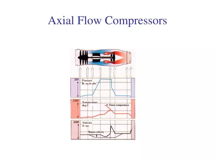
Axial Flow Compressors • Elementary theory
Axial Flow Compressors Comparison of typical forms of turbine and compressor rotor blades
Axial Flow Compressors Axial Flow Compressors Stage= S+R S: stator (stationary blade) R: rotor (rotating blade) First row of the stationary blades is called guide vanes • ** Basic operation • *Axial flow compressors: • series of stages • each stage has a row of rotor blades followed by a row of stator blades. • fluid is accelerated by rotor blades.
Axial Flow Compressors • In stator, fluid is then decelerated causing change in the kinetic energy to static pressure. • Due to adverse pressure gradient, the pressure rise for each stage is small. Therefore, it is known that a single turbine stage can drive a large number of compressor stages. • Inlet guide vanes are used to guide the flow into the first stage. Elementary Theory: Assume mid plane is constant r1=r2, u1=u2 assume Ca=const, in the direction of u. , in the direction of u.
Axial Flow Compressors Inside the rotor, all power is consumed. Stator only changes K.E.P static, To2=To3 Increase in stagnation pressure is done in the rotor. Stagnation pressure drops due to friction loss in the stator: C1: velocity of air approaching the rotor. : angle of approach of rotor. u: blade speed. V1: the velocity relative t the rotor at inlet at an angle 1 from the axial direction. V2: relative velocity at exit rotor at angle 2 determined from the rotor blade outlet angle. 2: angle of exit of rotor. Ca: axial velocity.
Axial Flow Compressors Two dimensional analysis: Only axial ( Ca) and tangential (Cw). no radial component
Axial Flow Compressors from velocity triangles assuming the power input to stage where or in terms of the axial velocity From equation (a)
Axial Flow Compressors Energy balance pressure ratio at a stage
Axial Flow Compressors Degree of reaction is the ratio of static enthalpy in rotor to static enthalpy rise in stage For incompressible isentropic flow Tds=dh-vdp dh=vdp=dp/ Tds=0 h=p/ ( constant ) Thus enthalpy rise could be replaced by static pressure rise ( in the definition of ) but generally choose =0.5 at mid-plane of the stage.
Axial Flow Compressors =0: all pressure rise only in stator =1: all pressure rise in only in rotor =0.5: half of pressure rise only in rotor and half is in stator. ( recommend design)
Axial Flow Compressors special condition =0 ( impulse type rotor) from equation 3 1=-2 , velocities skewed left, h1=h2, T1=T2 =1.0 (impulse type stator from equation 1) =1-Ca(tan1+tan2)/2u, 2=1 velocities skewed right, C1=C2, h2=h3T2=T3 =0.5 from 2
Axial Flow Compressors Three dimensional flow 2-D 1. the effects due to radial movement of the fluid are ignored. 2. It is justified for hub-trip ratio>0.8 3. This occurs at later stages of compressor. 3-D are valid due to 1. due to difference in hub-trip ratio from inlet stages to later-stages, the annulus will have a substantial taper. Thus radial velocity occurs. 2. due to whirl component, pressure increase with radius.
Axial Flow Compressors • Design Process of an axial compressor • (1) Choice of rotational speed at design point and annulus dimensions • (2) Determination of number of stages, using an assumed efficiency at design point • (3) Calculation of the air angles for each stage at the mean line • (4) Determination of the variation of the air angles from root to tip • (5) Selection of compressor blades using experimentally obtained cascade data • (6) Check on efficiency previously assumed using the cascade data • (7) Estimation on off-design performance • (8) Rig testing
Axial Flow Compressors • Design process: • Requirements: • A suitable design point under sea-level static conditions (with =1.01 bar and , 12000 N as take off thrust, may emerge as follows: • Compressor pressure ratio 4.15 • Air-mass flow 20 kg/s • Turbine inlet temperature 1100 K • With these data specified, it is now necessary to investigate the aerodynamic design of the compressor, turbine and other components of the engine. It will be assumed that the compressor has no inlet guide vanes, to keep weight and noise down. The design of the turbine will be considered in Chapter 7.
Axial Flow Compressors • Requirements: • choice of rotational speed and annulus dimensions; • determination of number of stages, using an assumed efficiency; • calculation of the air angles for each stage at mean radius; • determination of the variation of the air angles from root to tip; • investigation of compressibility effects
Axial Flow Compressors • Determination of rotational speed and annulus dimensions: • Assumptions • Guidelines: • Tip speed ut=350 m/s • Axial velocity Ca=150-200 m/s • Hub-tip ratio at entry 0.4-0.6 • Calculation of tip and hub radii at inlet • Assumptions Ca=150 m/s • Ut=350 m/s to be corrected to 250 rev/s
Axial Flow Compressors • Equations • continuity thus
Axial Flow Compressors • procedure
Axial Flow Compressors • From equation (a)
Axial Flow Compressors • Consider rps250 • Thus rr/rt=0.5, rt=0.2262, ut=2rt*rps=355.3 m/s Is ok. Discussed later. Results r-t=0.2262, r-r=0.1131, r-m=0.1697 m
Axial Flow Compressors • At exit of compressor
Axial Flow Compressors • No. of stages • To =overall = 452.5-288=164.5K • rise over a stage 10-30 K for subsonic • 4.5 for transonic • for rise over as stage=25 • thus no. of stages =164.5/25 - normally To5 is small at first stage de haller criterion V2/V1 >0.72 - work factor can be taken as 0.98, 0.93, 0.88 for 1st, 2nd, 3 rd stage and 0.83 for rest of the stages.
Axial Flow Compressors • Stage by stage design; • Consider middle plane • stage 1 • for no vane at inlet
Axial Flow Compressors • Angles check de Haller
Axial Flow Compressors • Second stage
Axial Flow Compressors • Stage 7 • At entry to the final stage the pressure and temperature are 3.56 bar and 429 K. the required compressor delivery pressure is 4.15*1.01=4.192 bar. The pressure ratio of the seventh stage is thus given by
Axial Flow Compressors • the corresponding air angles, assuming 50 per cent reaction, are then 1=50.98,
Design calculations using EES • "Determination of the rotational speed and annulus dimensions" • "Known Information" • To_1=288 [K]; Po_1=101 [kPa]; m_dot=20[kg/s]; U_t=350 [m/s] • $ifnot ParametricTable • Ca_1=150[m/s];r_r/r_t=0.5;cp=1005;R=0.287;Gamma=1.4 • $endif • Gamr=Gamma/(Gamma-1) • m_dot=Rho_1*Ca_1*A_1 "mass balance" • A_1=pi*(r_t^2-r_r^2) "relation between Area and eye dimensions" • U_t=2*pi*r_t*N_rps • C_1=Ca_1 • T_1=To_1-C_1^2/(2*cp) • P_1/Po_1=(T_1/To_1)^Gamr • Rho_1=P_1/(R*T_1) • $TabStops 0.5 2 in