Download
1 / 21
210 likes | 366 Views
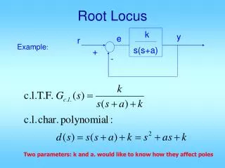
The root locus technique. Obtain closed-loop TF and char eq d(s) = 0 Re-arrange terms in d(s) by collecting those proportional to parameter of interest, and those not; then divide eq by terms not proportional to para. to get this is called the root locus equation

E N D
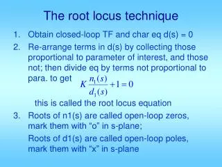
The root locus technique • Obtain closed-loop TF and char eq d(s) = 0 • Re-arrange terms in d(s) by collecting those proportional to parameter of interest, and those not; then divide eq by terms not proportional to para. to get this is called the root locus equation • Roots of n1(s) are called open-loop zeros, mark them with “o” in s-plane; Roots of d1(s) are called open-loop poles, mark them with “x” in s-plane
The “o” and “x” marks divide the real axis into several segments. If a segment has an odd total number of marks to its right, it is part of the root locus. High light it. If a segment has an even total number of marks, then it’s not part of root locus. For the high lighted segments, mark out going arrows near a pole (“x”), and incoming arrows near a zero (“o”).
Asymptotes:#asymptotes = # “x” - # “o” angles: 1 asymp: 180; 3 asymp: 180; +-60 2 asymp: +-90; 4 asymp: +-45; +-135 Meeting place on the real axis at:
Imaginary axis crossing point: • From d(s) = 0 • Form Routh Table • Set one row = 0 • Solve for K • Use the row above to aux eq A(s)=0 • Solution gives imag. axis crossing point +-jw • System oscillates at frequency w when K is equal to the value above
When two branches meet and split, you have breakaway points. They are double roots. Use these to solve for s and K: • Departure angles at complex pole p: fp Arrival anglesat complex zero z: fz
Char. poly. num: s+3 , zeros: -3 den: s(s+5)(s2+2s+2)(s+6) , poles:0, -5,-6,-1±j1 Asymptotes: #: n – m = 4 angles: ±45º, ±135º
Two branches coming out of -5 and -6 are heading to each other, and will and break away. Without actually calculating, we know the breakaway point is somewhere between -5 and -6. Since there are more dominant poles (poles that are closer to the jw axis), we don’t need to be bothered with computing the actual numbers for the break away point. Departure angle at p = -1+j is angle(-1+j+3)-angle(-1+j+0)-angle(-1+j+5)-angle(-1+j+4)+pi/2 ans = -0.8885 rad = -50.9061 deg
rlocus([1 3], conv([1 2 2 0],[1 11 30])) Hand sketch is close but departure angle is wrong! Also notice how I used “conv”.
Example: motor control The closed-loop T.F. from θr to θ is:
What is the open-loop T.F.? The o.l. T.F. of the system is: But for root locus, it depends on which parameter we are varying. • If KP varies, KD fixed, from char. poly.
The o.l. T.F. for KP-root-locus is the system o.l. T.F. In general, this is the case whenever the parameter is in the forward loop. • If KD is para, KP is fixedFrom
More examples No finite zeros, o.l. poles: 0,-1,-2 Real axis: are on R.L. Asymp: #: 3
-axis crossing: char. poly:
Example: Real axis: (-2,0) seg. is on R.L.
-axis crossing: char. poly:
-axis crossing: char. poly: