Download
1 / 27
290 likes | 469 Views
Reverend Thomas Bayes (1702-61). Bayes for Beginners. Stuart Rosen° and Elena Rusconi § °Department of Phonetics and Linguistics, UCL, § Institute of Cognitive Neuroscience, UCL MfD 15–II-2006. Overview of SPM Analysis. Statistical Parametric Map. Design matrix. fMRI time-series.

E N D
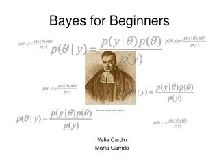
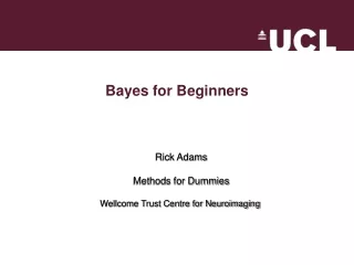
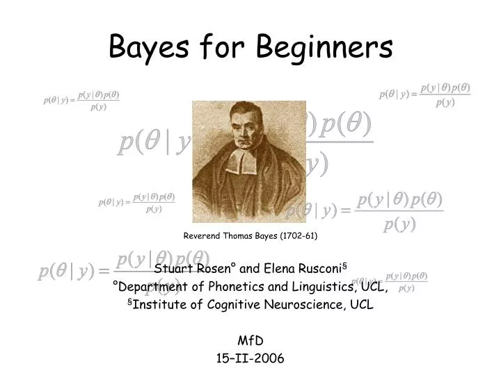
Reverend Thomas Bayes (1702-61) Bayes for Beginners Stuart Rosen° and Elena Rusconi§ °Department of Phonetics and Linguistics, UCL, §Institute of Cognitive Neuroscience, UCL MfD 15–II-2006
Overview of SPM Analysis Statistical Parametric Map Design matrix fMRI time-series Motion Correction Smoothing General Linear Model Parameter Estimates Spatial Normalisation Anatomical Reference
Spatial Normalisation - Overfitting Without Bayesian constraints, the non-linear spatial normalisation can introduce unnecessary warps. Affine registration. (2 = 472.1) Template image Non-linear registration without Bayes constraints. (2 = 287.3) Non-linear registration using Bayes. (2 = 302.7)
Bayes and image segmentation • Want to automatically classify regions into grey matter, white matter, CSF and non-brain tissue. • How do we use prior information? (probabilities of each voxel being of a particular type derived from a database of 152 scans) • Bayes!
A big advantage of a Bayesian approach • Allows a principled approach to the exploitation of all available data … • with an emphasis on continually updating one’s models as data accumulate • as seen in the consideration of what is learned from a positive mammogram
Bayesian Reasoning - Casscells, Schoenberger & Grayboys, 1978 - Eddy, 1982 • Gigerenzer & Hoffrage, 1995, 1999 • Butterworth, 2001 • Hoffrage, Lindsey, Hertwig & Gigerenzer, 2001 When PREVALENCE, SENSITIVITY, and FALSE POSITIVE RATES are given, most physicians misinterpret the information in a way that could be potentially disastrous for the patient.
Bayesian Reasoning ASSUMPTIONS 1% of women aged forty who participate in a routine screening have breast cancer 80% of women with breast cancer will get positive tests 9.6% of women without breast cancer will also get positive tests EVIDENCE A woman in this age group had a positive test in a routine screening PROBLEM What’s the probability that she has breast cancer?
Bayesian Reasoning ASSUMPTIONS 10 out of 1000 women aged forty who participate in a routine screening have breast cancer 800 out of 1000 of women with breast cancer will get positive tests 95 out of 1000 women without breast cancer will also get positive tests PROBLEM If 1000 women in this age group undergo a routine screening, about what fraction of women with positive tests will actually have breast cancer?
Bayesian Reasoning ASSUMPTIONS 100 out of 10,000 women aged forty who participate in a routine screening have breast cancer 80 of every 100 women with breast cancer will get positive tests 950 out of 9,900 women without breast cancer will also get positive tests PROBLEM If 10,000 women in this age group undergo a routine screening, about what fraction of women with positive tests will actually have breast cancer?
Bayesian Reasoning Before the screening: 100 women with breast cancer 9,900 women without breast cancer After the screening: A = 80 women with breast cancer and positive test B = 20 women with breast cancer and negative test C = 950 women without breast cancer and positive test D = 8,950 women without breast cancer and negative test Proportion of cancer patients with positive results, within the group of ALL patients with positive results: A/(A+C) = 80/(80+950) = 80/1030 = 0.078 = 7.8%
Compact Formulation C = cancer present, T = positive test p(A|B) = probability of A, given B, ~ = not PRIOR PROBABILITY p(C) = 1% CONDITIONAL PROBABILITIES p(T|C) = 80% p(T|~C) = 9.6% POSTERIOR PROBABILITY (or REVISED PROBABILITY) p(C|T) = ? PRIORS
Bayesian Reasoning Before the screening: 100 women with breast cancer 9,900 women without breast cancer After the screening: A = 80 women with breast cancer and positive test B = 20 women with breast cancer and negative test C = 950 women without breast cancer and positive test D = 8,950 women without breast cancer and negative test Proportion of cancer patients with positive results, within the group of ALL patients with positive results: A/(A+C) = 80/(80+950) = 80/1030 = 0.078 = 7.8%
Bayesian Reasoning Prior Probabilities: 100/10,000 = 1/100 = 1% = p(C) 9,900/10,000 = 99/100 = 99% = p(~C) Conditional Probabilities: A = 80/10,000 = (80/100)*(1/100) = p(T|C)*p(C) = 0.008 B = 20/10,000 = (20/100)*(1/100) = p(~T|C)*p(C) = 0.002 C = 950/10,000 = (9.6/100)*(99/100) =p(T|~C)*p(~C) = 0.095 D = 8,950/10,000 = (90.4/100)*(99/100) = p(~T|~C) *p(~C) = 0.895 Rate of cancer patients with positive results, within the group of ALL patients with positive results: A/(A+C) = 0.008/(0.008+0.095) = 0.008/0.103 = 0.078 = 7.8%
-----> Bayes’ theorem p(T|C)*p(C) p(C|T)= ______________________ P(T|C)*p(C)+p(T|~C)*p(~C) A A + C
Comments • Common mistake: to ignore the prior probability • The conditional probability slides the revised probability in its direction but doesn’t replace the prior probability • A NATURAL FREQUENCIES presentation is one in which the information about the prior probability is embedded in the conditional probabilities (the proportion of people using Bayesian reasoning rises to around half). • Test sensitivity issue (or: “if two conditional probabilities are equal, the revised probability equals the prior probability”) • Where do the priors come from?
-----> Bayes’ theorem p(X|A)*p(A) p(A|X)= ______________________ P(X|A)*p(A)+p(X|~A)*p(~A) Given some phenomenon A that we want to investigate, and an observation X that is evidence about A, we can update the original probability of A, given the new evidence X.
Bayes’ Theorem for a given parameter p (data) = p (data)p () / p (data) 1/P (data) is basically a normalizing constant Posteriorlikelihood x prior The prior is the probability of the parameter and represents what was thought before seeing the data. The likelihood is the probability of the data given the parameter and represents the data now available. The posteriorrepresents what is thought given both prior information and the data just seen. It relates the conditional density of a parameter (posterior probability) with its unconditional density (prior, since depends on information present before the experiment).
lpost-1 ld-1 lp-1 Mp Mpost Md Posterior Probability Distribution precision = 1/2 Likelihood: p(y|) = N(Md, ld-1) Prior: p() = N(Mp, lp-1) Posterior: p(|y)∝p(y|)*p() = N(Mpost, lpost-1) lpost=ld + lpMpost= ld Md + lp Mp lpost
Activations in fMRI…. • Classical • ‘What is the likelihood of getting these data given no activation occurred?’ • Bayesian option (SPM2) • ‘What is the chance of getting these parameters, given these data?
What use is Bayes in deciding what brain regions are active in a particular study? • Problems with classical frequentist approach • All inferences relate to disproving the null hypothesis • Never fully reject H0, only say that the effect you see is unlikely to occur by chance • Corrections for multiple comparisons • significance depends on the number of contrasts you look at • Very small effects can be declared significant with enough data • Bayesian Inference offers a solution through Posterior Probability Maps (PPMs)
SPMs and PPMs PPMs: Show activations of a given size SPMs: show voxels with non-zero activations
PPMs Disadvantages Advantages Computationally demanding (priors are determined empirically) Utility of Bayesian approach is yet to be established One can infer a cause DID NOT elicit a response SPMs conflate effect-size and effect-variability
Frequentist vs. Bayesian by Berry 1. Probabilities of data vs. probabilities of parameters (& also data). 2. Evidence used: • Frequentist measures specific to experiment. • Posterior distribution depends on all available information. Makes Bayesian approach appealing, but assembling, assessing, & quantifying information is work.
3. Depend on probabilities of results that could occur vs. did occur: • Frequentist measures (e.g., p values, confidence intervals) incorporate probabilities of data that were possible but did not occur. • Posterior depends on data only through the likelihood, which is calculated from observed data. 4. Flexibility: • Frequentist measures depend on design; require that design be followed. • Bayesian view: update continually as data accumulate (only requirement is honesty). Sample size: need not choose in advance. Weigh costs/benefits; decide whether to start experiment. After experiment starts, decide whether to continue—stop at any time, for any reason.
5. Decision making • Frequentist: historically avoided. • Bayesian: tailored to decision analysis; losses and gains considered explicitly.
References • Statistics: A Bayesian Perspective D. Berry, 1996, Duxbury Press. • excellent introductory textbook, if you really want to understand what it’s all about. • http://ftp.isds.duke.edu/WorkingPapers/97-21.ps • “Using a Bayesian Approach in Medical Device Development”, also by Berry • http://www.pnl.gov/bayesian/Berry/ • a powerpoint presentation by Berry • http://yudkowsky.net/bayes/bayes.html • Extremely clear presentation of the mammography example; highly polemical and fun too! • http://www.stat.ucla.edu/history/essay.pdf • Bayes’ original essay • Jaynes, E. T., 1956, `Probability Theory in Science and Engineering,' (No. 4 in `Colloquium Lectures in Pure and Applied Science,' Socony-Mobil Oil Co. USA. http://bayes.wustl.edu/etj/articles/mobil.pdf • A physicist’s take on Bayesian approaches. Proposes an interesting metric of probability using decibels (yes, the unit used for sound levels!). • http://www.sportsci.org/resource/stats/ • a skeptical account of Bayesian approaches. The rest of the site is very informative and sensible about basic statistical issues.
Bayes’ ending Bunhill Fields Burial Ground off City Road, EC1