Download
1 / 21
220 likes | 417 Views
Bayes for beginners. Claire Berna. Lieke de Boer. Methods for dummies 27 February 2013. Bayes rule Given marginal probabilities p(A ), p(B ), and the joint probability p(A,B ), we can write the conditional probabilities:. This is known as the product rule . .

E N D
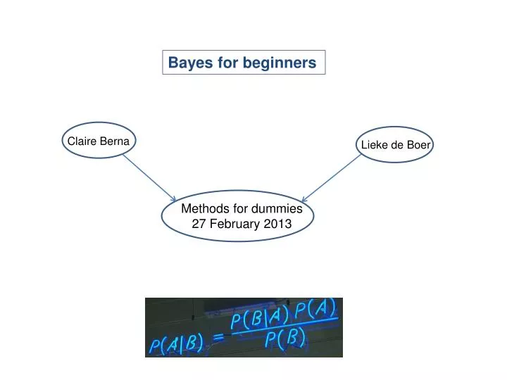
Bayes for beginners Claire Berna Lieke de Boer Methods for dummies 27 February 2013
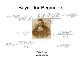
Bayes rule Given marginal probabilities p(A), p(B), and the joint probability p(A,B), we can write the conditional probabilities: This is known as the product rule. Eliminating p(A,B) gives Bayes rule: p(A|B) p(B) p(A,B) p(A,B) p(B/A) = p(B|A) = p(A|B) = p(A) p(B) p(A)
Example: The lawniswet : we assume that the lawniswetbecauseit has rainedovernight: How likelyisit? p(w|r) : Likelihood Whatis the probabilitythatit has rainedovernight giventhis observation? p(r|w): Posterior: How probable isourhypothesisgiven the observedevidence? P(r): Prior: Probability to rain on thatday. How probable wasourhypothesisbeforeobserving the evidence? p(w) : Marginal: how probable is the new evidenceunder all possible hypotheses? p(w|r) p(r) p(r|w) = p(w)
Example: The probability p(w) is a normalisation term and can be found by marginalisation. p(w=1) =∑ p(w=1, r) r = p(w=1,r=0) + p(w=1,r=1) = p(w=1|r=0)p(r=0) + p(w=1|r=1)p(r=1) p(w=1 | r=1) = 0.95 p(w=1 | r=0) = 0.20 • p(r = 1) = 0.01 This isknown as the sumrule = 0.046 p(w|r) p(r) p(w=1|r=1) p(r=1) p(w=1|r=1) p(r=1) p(r=1|w=1) = p(r|w) = p(r=1|w=1) = p(w=1|r=0)p(r=0) + p(w=1|r=1)p(r=1) p(w) p(w=1)
Did I Leave The Sprinkler On ? A single observation with multiple potential causes (not mutually exclusive). Both rain, r , and the sprinkler, s, can cause my lawn to be wet, w. p(w,r ,s) = p(r )p(s)p(w|r,s) Generative model
Did I Leave The Sprinkler On ? The probability that the sprinkler was on given i’ve seenthe lawn is wet is given by Bayes rule = • where the joint probabilities are obtained from marginalisationand from the generative model: p(w, r , s) = p(r ) p(s) p(w|r,s) • p(w = 1, s = 1) = ∑1p(w = 1,r ,s = 1) = p(w=1, r=0, s=1) + p(w=1, r=1, s=1) • r=0 • = p(r=0) p(s=1) p(w=1|r=0, s=1) + p(r=1) p(s=1) p(w=1|r=1, s=1) • p(w = 1, s = 0) = ∑1p(w = 1,r ,s = 0) = p(w=1, r=0, s=0) + p(w=1, r=1, s=0) • r=0 • = p(r=0) p(s=0) p(w=1|r=0, s=0) + p(r=1) p(s=0) p(w=1|r=1, s=0) p(w=1|s=1) p(s=1) p(w = 1, s = 1) + p(w = 1, s = 0) p(w=1|s=1) p(s=1) p(s=1|w=1) = p(w=1)
Numerical Example • Bayesian models force us tobe explicit about exactly whatit is we believe. • p(r = 1) = 0.01 • p(s = 1) = 0.02 • p(w = 1|r = 0,s = 0) = 0.001 • p(w = 1|r = 0,s = 1) = 0.97 • p(w = 1|r = 1,s = 0) = 0.90 • p(w = 1|r = 1,s = 1) = 0.99 • These numbers give • p(s = 1|w = 1) = 0.67 • p(r = 1|w = 1) = 0.31
Look next door Rain r will make my lawn wet w1 andnextdoorsw2 whereas the sprinkler s only affects mine. p(w1, w2, r, s) = p(r )p(s)p(w1|r,s)p(w2|r )
After looking next door Use Bayes rule again with joint probabilities from marginalisation p(w1= 1, w2= 1,s = 1) = ∑1 p(w1 = 1, w2 = 1, r , s = 1) r=0 p(w1= 1, w2= 1,s = 0) =∑1 p(w1 = 1;w2 = 1; r ; s = 0) r=0 p(w1=1, w2=1, s=1) p(s=1|w1=1, w2=1) = p(w1= 1, w2 = 1, s = 1) + p(w1= 1, w2 = 1, s = 0)
Explaining Away • Numbers same as before. In addition • p(w2 = 1|r = 1) = 0.90 • Now we have • p(s = 1|w1 = 1, w2 = 1) = 0.21 • p(r = 1|w1 = 1, w2 = 1) = 0.80 • The fact that my grass is wet has been explained away by • the rain (and the observation of my neighbours wet lawn).
The CHILD network Probabilistic graphical model for newborn babies with congenital heart disease Decision making aid piloted at Great Ormond Street hospital (Spiegelhalter et al. 1993).
When comparing two models Bayesian inference in neuroimaging A > B ? • When assessing the inactivity of a brain area P(H0)
• invert model (obtain posterior pdf) • define the null, e.g.: • define the null, e.g.: • estimate parameters (obtain test stat.) • apply decision rule, i.e.: • apply decision rule, i.e.: if then reject H0 if then accept H0 Bayesian PPM classical approach Assessing inactivity of brain area
Bayesian paradigm likelihood function • GLM: y = f(θ) + ε • From the assumption: • noise is small • Create a likelihood function with a fixed θ:
So θ needs to be fixed... priors Probability of θ, depends on: • model you want to compare • data • previous experience Likelihood: Prior: Bayes' rule:
Bayesian inference Precision = 1/variance
Bayesian inference forward/inverse problem likelihood posterior distribution
Bayesian inference Occam's razor ‘The hypothesis that makes the fewest assumptions should be selected’ ‘Plurality should not be assumed without necessity’
hierarchy causality Bayesian inference Hierarchical models
References: • - Will Penny’s course on Bayesian Inference, FIL, 2013 • http://www.fil.ion.ucl.ac.uk/~wpenny/bayes-inf/ • - J. Pearl (1988) Probabilistic reasoning in intelligent systems. • San Mateo, CA. Morgan Kaufmann. • Previous MfD presentations • Jean Daunizeau’s SPM course a the FIL Thanks to Ged for his feedback!