General Relativity Physics Honours 2009

General RelativityPhysics Honours 2009 Prof. Geraint F. Lewis Rm 560, A29 gfl@physics.usyd.edu.au Lecture Notes 4

Gravitational Lensing There are many astrophysical applications using what we have already learnt. Here we will examine two; gravitational lensing and relativistic accretion disks. Given that massive objects can deflect the path of a beam of light, this means that objects can behave as a gravitational lens. Such lenses resemble glass lenses in many ways, giving multiple images which can be magnified. Chapter 11

Accretion Disks Accretion disks are important in astrophysics as they efficiently transform gravitational potential energy into radiation. Accretion disks are seen around stars, but the most extreme disks are seen at the centre of quasars. These orbit black holes with masses of ~106-9 M, and radiate up to 1014 L, outshining all of the stars in the host galaxy. If we assume the black hole is not rotating, we can describe its spacetime with the Schwarzschild metric and make predictions for what we expect to see.

Accretion Disks Suppose we have radiating material orbiting a black hole. The photons leave the disk and are received by a distant observer. How much redshifting of the photons does the observer see?

Accretion Disks How fast is the material orbiting? Assuming circular orbits So we write the 4-velocity of the emitting matter to be And using the normalization of the 4-velocty

Accretion Disks We can now us the Killing vector conserved quantities; Remember, the conserved quantities and the impact parameter are related via

Accretion Disks Remember we are in a plane where =/2. What redshift do we see? Let’s consider the matter moving transversely to the line-of-sight. For these, b=0 and so So, there is no Doppler component. What about the matter moving directly towards or away from the observer? Now we explicitly need to consider the value of b

Accretion Disks Remembering that photons are null And so The resultant frequency ratio is

Accretion Disks For small values of M/r then where

Accretion Disks Accretion disks are hot an emit in highly ionized species. Remembering that the radius for the last stable orbit occurs at r=6M, the maximum redshift for an edge-on disk is For a face-on disk, this is ~0.7. Above is the X-ray spectrum of the 6.4keV Fe line in a Seyfert galaxy. The solid line is a fit to the data using a relativistic accretion disk seen at 30o. The extent of the redshift reveals this must be a black hole.

Black Holes We have seen previously that something weird happens when we fall towards the origin of the Schwarzschild metric; while the proper motion for the fall is finite, the coordinate time tends to r=2M as t->∞. Clearly, there is something weird about r=2M (the Schwarzschild radius) for massive particles. But what about light rays? Remembering that light paths are null so we can calculate structure of radial light paths. Chapter 12

Black Holes We can calculate the gradients of light rays from the metric Again, light curves tell us about the future of massive particles. Clearly the light cones are distorted, and within r=2M all massive particles are destined to hit the origin (the central singularity). In fact, once within this radius, a massive particle will not escape and is trapped (and doomed)! But how do we cross from inside to outside?

Eddington-Finkelstein While Eddington figured out the solution in the early 1900s, but it was Finkelstein in the late 1950s who rediscovered the answer. Basically, we will just make a change of coordinates; And the Schwarzschild metric can be written as The geometry is the same, but the metric now contains off-axis components. But notice now that the metric does nothing weird at r=2M (but still blows up at r=0).

Eddington-Finkelstein Light rays are still null, so we can find the light cones Clearly, v=const represents a null geodesic (and these are ingoing rays). There is another that can be integrated; http://casa.colorado.edu/~ajsh/ So, the change in coordinates removes the coordinate singularity and now light (and massive particles) happily fall in.

Eddington-Finkelstein To create this figure, we define a new time coordinate of the form; This straightens in-going light rays (making it look like flat space time). However, outgoing light rays are still distorted.

White Holes Another coordinate transformation can straighten outgoing light rays. The result is a white hole and massive particle at r<2M are destined to be ejected and cannot return. Note that while this is still the Schwarzschild solution, this behaviour is not seen in the original solution.

Collapse to a Black Hole Consider the collapse of a pressureless (dust) star. The surface of the will collapse along time-like geodesics. We know that the proper time taken for a point to collapse to r=0 is While the Schwarzschild metric blows up at the horizon, the E-F coordinates remain finite and you can cross the horizon. Once across the horizon, the time to the origin is Which is 10-5s for the Sun. Surfaces B12.2

Collapse to a Black Hole Remember that in E-F coordinates, outgoing light rays move along geodesics where Let’s consider an emitter at (vE,rE) and receiver at (vR,rR). If the receiver is at large distances, then the log term can be neglected. When the emitter is close to r=2M the log term dominates. For the distant observer then Where t is the Schwarzschild time coordinate (which will equal the proper time of the observer as the spacetime far from the hole is flat).

Collapse to a Black Hole Keeping the dominant terms, the result is As rE2M, tR∞; Photons fired off at regular intervals of proper time are received later and later by the observer. These photons are also redshifted. If the photons are emitted at regular intervals of (proper time) then

Collapse to a Black Hole Remembering that the frequency of the emitted and received photons are inversely related to the ratio of the emitted and received time between photons, then So the distant observer sees the surface of the star collapsing, but as it approaches r=2M it appears to slow and the received photons become more and more redshifted. The distant observer never sees the surface cross the Schwarzschild radius (or horizon) although we see from the E-F coordinates, the mass happily falls through.

Kruskal-Szekeres We can take the game of changing coordinates even further with Kruskal-Szekeres coordinates. Starting again with the Schwarzschild metric, and keeping the angular coordinates unchanged, the new coordinates are given by Where c & s are cosh & sinh with the first combination used for r>2M and the second for r<2M. We also find that

Kruskal-Szekeres The resultant metric is of the form

Kruskal-Szekeres Lines of constant t are straight, while those at constant r are curves. Light cones are at 45o, as in flat spacetime. We have our universe, plus a future singularity (black hole) and past singularity (white hole). There also appears to be another universe over to the left.

Kruskal-Szekeres We can examine the radial infall of matter in these coordinates. The distant observer moves along a line of constant radius, while the matter falls in emitting photons. Again, the distant observer sees the photons arriving at larger intervals and never sees the matter cross the horizon. Note that once inside the horizon, the matter must hit the central singularity.

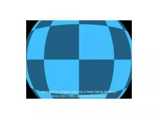
Penrose Penrose mapped the Kruskal coordinates further, such that now we get two entire universes on a single page. This is an example of maximal compactification.

Astrophysical Black Holes Unfortunately, we don’t have time to cover astrophysical black holes in the lectures, but you should read through Chapter 12 of the textbook. You should ensure you read in detail Section 13.3 which explains how black holes can evaporate via Hawking radiation. Chapter 13

Rotation So far, we have considered the motion of point like particles through spacetime. These travel along timelike (massive) or null (massless) geodesics; This equation actually parallel transports the tangent vector to the geodesic (the 4-velocity) along the path. Clearly, in flat Minkowski spacetime, the Christoffel symbols are zero. Other vectors can undergo parallel transport. The spin of a gyroscope can be represented as a spacelike spin 4-vector. Chapter 14

Rotation In our rest frame, And the 4-spin and 4-velocity are orthogonal. However, this must hold in all frames. The 4-spin is parallel transported along the geodesic using As we will see later, this is related to the covariant derivative, and the Christoffel symbols take into account the change in the coordinates over the manifold. In flat space, the spin of the gyroscope remains fixed. What about curved spacetime?

Rotation Let’s consider a gyroscope orbiting in the static Schwarzschild metric. We will see that General Relativity predicts that, relative to the distant stars, the orientation of the gyroscope will change with time. This is geodetic precession. If the gyroscope is on a circular orbit then And so the 4-velocity is given by (Remember we are orbiting in a plane where =/2)

Rotation We can use the orthogonality to find And solving we find We can use the Christoffel symbols for the Schwarzschild metric and the gyroscope equation to find;

Rotation Combining these, we can derive the equation This is just the usual wave equation with a frequency Clearly, there is something weird here. The components of the spin vector change with time, but the frequency is not the same as the orbital frequency. So, the spin angle and the orbital frequency are out of phase.

Rotation The solution to these equations are quite straight-forward and Where s.s=s2*. Let’s consider t=0 and align the spin along the radial direction and we need to look at the orthonormal frame of the observer; as the metric is diagonal, we can define the radial orthonormal vector is

Rotation The period of the orbit is P=2/ and therefore the component of spin in the radial direction after one orbit is So, after each orbit, the direction of the spin vector has been rotated by This is the shift for a stationary observer at this point in the orbit. We could also set up a comoving observer at this point (orbiting with the gyro) but the radial component of the spin vector would be the same.

Rotation For small values of M/R the angular change is For a gyroscope orbiting at the surface of the Earth, this corresponds to While small, this will be measured by Gravity Probe B. What would you expect if you were in an orbiting laboratory with windows that opened once per year?

Slowly Rotating Spacetime • So far, our massive objects have been static, but what if the body is rotating? We won’t have time to consider the derivation of the effect in general, but you can read it in Section 23.3. For a slowly rotating spherical mass Where J is the angular momentum of the mass. Hence the form of the metric is deformed, but what is the effect of this distortion? Firstly, lets consider this metric in cartesian coordinates;

Slowly Rotating Spacetime Let’s drop a gyro down the rotational axis. We can approximate the Schwarzschild metric as being flat (as contributing terms would be c-5). For our motion down the z-axis (rotation axis) then The non-zero Christoffel symbols for our flat + slow rotation metric are simply When evaluated on the z-axis and retaining the highest order terms. From this, we can use the gyroscope equation to show;

Slowly Rotating Spacetime Again, we have a pair of equations that show that the direction of the spin vector change with time with a period of This is Lense-Thirring precession. At the surface of the Earth this has a value of While small, this will be observable by GP-B.

Rotating Black Holes Unfortunately, we will not get time in this course to look at general black holes. Here we will just review the basic properties. If a black hole is rotating, its spacetime geometry is described by the Kerr metric. where These are Boyer-Lindquist coordinates. This is asymptotically flat and the Schwarzschild metric when a=0.

Rotating Black Holes • We can analyze particle motion in this metric using the same approach as we have used previously. The horizon is flattened and the singularity is distorted into a ring. http://www.engr.mun.ca/~ggeorge/astron/shad/index.html

Charged Black Holes • The only thing left that can influence the form of black holes is charge (black holes have no hair). The geometry of a charged black hole is described by the Reissner-Nordstrom metric. Where eis the charge of the black hole. Again, when the charge is zero, we recover the Schwarzschild solution. Again, the metric results in weird structure not seen in the simple solution. If 2>m2, then we have a central singularity but no shielding horizon, it is naked.

General Relativity Physics Honours 2009