Download
1 / 52
520 likes | 642 Views
General Relativity Physics Honours 2005. Dr Geraint F. Lewis Rm 557, A29 gfl@physics.usyd.edu.au. The Field Equations. It is time to look at the “source” of the metric and this involves understanding the field equations of General Relativity.

E N D
General RelativityPhysics Honours 2005 Dr Geraint F. Lewis Rm 557, A29 gfl@physics.usyd.edu.au
The Field Equations It is time to look at the “source” of the metric and this involves understanding the field equations of General Relativity where T is the stress-energy tensor and the R terms are the Ricci tensor and scalar. The left terms contain the metric (and its derivatives) whereas the right describes the distribution of energy. The field equations are ten 2nd order PDEs which must be solved to determine the metric for a particular energy distribution.
Manifolds (Ch 5) General relativity is based upon non-Euclidean geometry. To understand this, we must consider the concept of a manifold. Crudely speaking a manifold is an object which is locally isomorphic to a piece of n-dimensional euclidian space Rn . Hence, in a small region about any point it can be parameterized by n coordinates. If each point has a unique set of coordinates, then the coordinate system is non-degenerate.
Manifolds A non-degenerate coordinate system cannot always be extended over the manifold and generally overlapping coordinate patches are used. Hence, we need to understand coordinate transforms to take us between the patches on a manifold. Example: A plane can be covered with a single non-degenerate coordinate system (i.e. cartesian), but can also be covered with polar coordinates which are degenerate at the origin (i.e. is undefined). Example: A sphere cannot be covered with a single non-degenerate coordinate system.
Coordinate Transforms Suppose a point has coordinates xa (a=1,…,n) in one set of coordinates. In a passive coordinate transform we can find x’ain a new coordinate system with the new coordinates being functions of the old coordinates (i.e. x’a = x’a (x)). Example: cartesian coordinates can be expressed as a function of spherical polar coordinates.
Coordinate Transforms Differentiating the mapping between coordinate systems give the transformation matrix The determinant J’ of the matrix is the Jacobian and if it is non-zero we can define the inverse transform xa=xa(x’). The total differential is then
Coordinate Transforms The cartesian and spherical polar example; The Jacobian is J’=r2 sinand Etc.
Contravariant Tensors Definition: tensors are quantities that satisfy certain transformation laws. Tensors contain vectors and scalars as special cases. We just saw the transformation for the infinitesimal total differential vector. This is a contravariant vector (or tensor of rank 1); i.e. the quantity Xaat a point which transforms as The infinitesimal vector dxaand the tangent vector dxa/du to the curve x(u) are contravariant vectors.
Contravariant Tensors We can generalize this idea to higher tensors. A contravariant tensor of rank 2 is defined to be the object at point P that transforms as Higher order tensors as defined analogously. A scalar is a contravariant tensor of rank 0 and is invariant under a coordinate transformation.
Covariant Tensors Consider the function (xb). If we regard the xbas functions of the x’athen; Thus, the gradient operator / xb transforms in a different way to contravariant tensors. Hence a covariant tensor of rank 1 can be defined as
Mixed Tensors A mixed tensor can be defined such as which is contravariant rank 1 and covariant rank 2 and is called a type (1,2). An example of a mixed rank tensor is the conductivity tensor (s) that relates the th component of the 3-current j to the th component of the electric field E.
Tensor Fields A tensor is defined at a particular point. A tensor field associates a tensor at each point on a manifold. Rank 0: potential energy Rank 1: electric field Rank 2: conductivity Remember, transformations between coordinate systems depend upon the location on the manifold.
Elementary Operations Tensors can only be added to, or subtracted from, tensors of the same type. Scalar multiplication of a tensor results in a tensor of the same type. Note, indicies must match up in every term. A tensor can be symmetrized or antisymmetrized to give
Elementary Operations The alternating sum has a positive sign for even permutations of ai and negative signs for odd permutations. We can define a tensor multiplication such that
Contraction We will see contraction throughout the course. The idea is to sum over a pair of contra and covariant indicies. Hence, Xabcd can be contracted on a and b through Hence a tensor of type (1,3) contracts to a tensor of type (0,2). For example the left is type (0,1), while the right is (1,2) contracted to (0,1).
Index-Free Notation Section 5.9 discusses an index free interpretation of tensors. We will not consider them further here, but you should be familiar with the concept (although most discussions of general relativity appear to prefer the indexed version of tensors).
Tensor Calculus We need to consider the differentiation of tensors. This would involve an entire formal course, but here we will focus on issues we need in General Relativity. We denote the partial derivative of a contravariant tensor as How does this quantity transform?
Tensor Calculus The partial derivative of a tensor is This is not a tensor (why?)! This is not surprising as the limiting process to obtain a partial derivative involves evaluating the tensor at two different places.
Lie Derivative Consider a congruence of curves such that a unique curve goes through each point on the manifold. We can parameterize one of these curves as xa=xa(u) and can define a field of tangent vectors Conversely, a non-zero vector field yields a unique congruence of curves over at least a subset of the manifold (Fig 6.1 & 6.2).
Lie Derivative Suppose the field Xais given, and we can construct the corresponding congruence of curves. To differentiate the tensor T at the point P we drag T along the curve through P to a neighbouring point Q. The derivative therefore compares the dragged tensor with the tensor evaluated at Q in the limits that Q! P. 1) If the coordinates at P are xa, those at Q are for a small displacement u along the curve though P.
Lie Derivative 2) We can treat the shift from xa to x’a as an active coordinate transformation with 3) Consider the tensor Tab. The components of the dragged along tensor at Q are
Lie Derivative 4) The value of the tensor at Q can be obtained by Taylor-expanding T about P to the same order 5) Define the Lie Derivative of Tab with respect to Xa as
Lie Derivative We can always introduce a coordinate system such that Then the Lie derivative reduces to In this special coordinate system, the Lie derivative reduces to an ordinary directional derivative.
Lie Derivative • Linear • Satisfies the product rule • Preserves tensor type • Is the directional derivative for a scalar field • The Lie derivative for a general tensor field is with a negative term for each contravariant index, and a positive term for each covariant index.
Covariant Derivative Now we have the Lie derivative, we need to another (more useful) form of tensor derivative. Again, we will consider a contravariant vector field Xa(x) evaluated at Q(x+ x) near P(x). Taylor’s theorem gives Again the difference is not tensorial as we are subtracting tensors at two different points. We will define the covariant derivative by comparing X(x+ x) with a vector which is in some sense parallel to the one at P.
Covariant Derivative Writing the parallel vector as To lowest order the barred term must be linear in Xaand dxbsuch that where the properties of have yet to be defined.
Covariant Derivative We can define the covariant derivative to be Clearly the Gterm (the affine connection) does not transform like a tensor. This is not surprising considering that its role is to compensate for non-tensorial aspects of the derivative. The covariant derivative of a scalar satisfies
Covariant Derivative Furthermore, for a covariant vector and in general Throughout this course we will restrict ourselves to symmetric connections such that
Covariant Derivative When considering the derivatives of the components of a tensor, the affine connection can be seen to include contributions from changes in the tensor, plus contributions from the twisting and turning of the coordinates in general curvilinear coordinates. When we differentiate ajwe are really differentiating the vector ajej, where ejis the jthunit vector of the coordinate system.
Affine Geodesics Introducing the notation which represents the covariant derivative contracted with X; cf. the usual directional derivative We can define the absolute derivative to be
Affine Geodesics The tensor is said to be parallel-transported along the curve if its absolute derivative vanishes i.e we hold it locally as constant as possible along the congruence curve defined X. As an example, we could compare a vector to a gyroscope also taken along the curve. An affine geodesic is a curve along which its own tangent vector is propagated parallel to itself, or the straightest possible curve
Affine Geodesic This is equivalent to (exercise) If we parameterize the curve such that (u) vanishes, then the tangent vector is parallely transported (or propagated) along the curve onto itself.
Affine Geodesic The affine parameter s is only defined up to an affine transformations! s + . Here, and are constants. Hence, we can calculate the affine length along a geodesic as Note that we cannot compare lengths along different geodesics without a metric.
Riemann Tensor Generally, covariant derivatives do not commute; (assuming that the terms are symmetric). The Riemann Tensor is related to the curvature of a manifold and vanishes when the manifold is “flat” (i.e. where the covariant derivatives commute). We can use this as the definition of flat.
Affine Flatness • Properties of a manifold; • There exists a special coordinate system in which the connection coefficients vanish everywhere (affine flat). • Manifold is integrable if vectors transported along various paths between two points are transported to the same vector. • Manifold is integrable iff its Riemann tensor vanishes everywhere. • Manifold is affine flat iff its connection is symmetric & integrable. • Manifold is flat iff Riemann tensor vanishes everywhere.
Geodesic Coordinates While “affine flatness” is a global concept, we can also describe a local flatness. The Geodesic Coordinates are those in which the connection coefficients vanish, but not their derivatives (or the curvature tensor). This yields ’abc|P = 0. This coordinate system is the flattest looking one at the points P and for a 2-D surface this would represent the tangent plane at P. More generally it represents a tangent space.
Metric: Reminder The square of the infinitesimal distance between two points xa and xa + dxa is where the metric tensor gab is a symmetric tensor that defines the metric. Furthermore, we define the norm of a vector X
Metric: Reminder The metric is non-singular if the determinant is non-zero and an inverse exists so The metric tensor can be used to raise and lower indicies on tensors by defining In general;
Metric Flatness A metric is flat if there exists a coordinate system in which the metric tensor reduces to a diagonal form The metric tensor is flat iff it Riemann tensor vanishes. (Note the signature of the metric in this form is the sum of the diagonal components).
Metric Geodesic The curve with maximum or minimum (i.e. stationary) between two points is the metric geodesic (Ch 7) with (Note that this is a particular case of a more general argument. Affine and metric geodesics coincide only if the connection is symmetric i.e. torsion free. Read the details in Ch 6).
Curvature Tensor The curvature tensor Rabcd embodies the curvature of the metric. As we have seen, this quantity depends upon the metric, as well as its first and second derivatives. Hence, Rabcd is really a series of coupled differential equations (but what is it equal to?) On an n-dimensional manifold, this tensor has n4components, but it possesses a number of symmetries which reduces the number of independent components.
Curvature Tensor These symmetries are (Pg 86) This reduces the number of independent components to Hence, for the case we are interested in (n=4) this reduces the number of independent components from 256 to 20!
Curvature Tensor Rabcd also satisfies the Bianchi identities Two important quantities are contractions of the curvature tensor
Einstein Tensor The Ricci tensor and scalar are combined to give another symmetric tensor, the Einstein Tensor In terms of relativity, this is the most useful representation of the curvature tensor & satisfies the contracted Bianchi identities
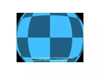
Spheres & Cylinders Remember, what we have seen is related to non-Euclidean geometry, and is not specific to relativity! We can consider two simple examples, the sphere and the cylinder, to explore these concepts. In the following, the shapes may be three dimensional, but the manifold refers to only the two dimensional surfaces. The third dimension only aids visualization. The higher dimensions required to visualize 4-d manifolds in relativity just make your head hurt!
Spheres & Cylinders Coordinates on a sphere can be labeled with and . The line element on a sphere is given by Remember, a 2-d being on the surface of the sphere has no physical concept of r. The metric is simply given by
Spheres & Cylinders Given that det(gab) = r4 sin2 0 the metric is non-singular except at = 0 & . Hence We can now calculate the connections i.e. two independent coefficients.
Spheres & Cylinders The 24=16 element Riemann tensor is (all other cmpts are zero) Lowering the first index gives and the symmetries noted earlier are verified. The tensor does not vanish, and so the metric is not flat. Neither is it affine flat or integrable.
Spheres & Cylinders The components of the Ricci tensor and scalar are The resulting Einstein tensor is Gab = 0 (note that in n>2 this can only happen if Rab=0).
Spheres & Cylinders The geodesic equations are Rotating to =p/2 and taking d/ds=0 initially These are great circle paths over the sphere.