General Relativity Physics Honours 2007

General RelativityPhysics Honours 2007 A/Prof. Geraint F. Lewis Rm 557, A29 gfl@physics.usyd.edu.au Lecture Notes 4

Schwarzschild Geometry When faced with the field equations, Einstein felt that it analytic solutions may be impossible. In 1916, Karl Schwarzschild derived the spherically symmetric vacuum solution, which describes the spacetime outside of any spherical, stationary mass distribution; This is in Geometrized units, where G=c=1. Note, that the geometrized mass has units of length and so the curved terms in the invariant above are dimensionless. Ch. 9

Schwarzschild Geometry An examination of the Schwarzschild metric reveals; Time Independence: The metric has the same form for all values of t. Hence we have a Killing vector; Spherical Symmetry: This implies further Killing vectors, including one due to the independence of ; Weak Field Limit: When M/r is small, the Schwarzschild metric becomes the weak field metric we saw earlier.

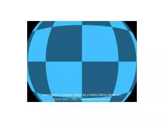
Schwarzschild Geometry Something clearly goes wrong at r=0 (the central singularity) and r=2M (Schwarzschild radius or singularity). More on this later. Remember: the (t,r,,) in this expression are coordinates and r is not the distance from any centre! If we choose a t=constant & r=constant we see the resulting 2-dimensional surface is a sphere (in 3-dimensions). So we can simply relate the area to r, but not the volume!

Particle Orbits Massive particles follow time-like geodesics, but understanding their motion is aided by identifying conserved quantities. Given our two Killing vectors we obtain At large r the first conserved quantity is the energy per unit mass in flat space; While the second is the angular momentum per unit mass.

Particle Orbits The conservation of l implies particles orbit in a plane. Consider an time-like geodesic passing through the point =0, with d/d=0. The conservation of l ensures d/d=0 along the geodesic and so the particle remains in the plane =0. But the spherical symmetry implies this is true for all orbits. Hence we will consider equatorial orbits with =/2 and u=0. Defining the 4-velocity of the particle to be

Particle Orbits Substituting in our conserved quantities we get where This result differs from the Newtonian picture (found in any classical mechanics text) with the addition of the r-3 term in the potential! At large r the orbits become more Newtonian. Remember, while orbits are closed in r-1 potentials, they are not in general potentials.

Particle Orbits Considering the relativistic and Newtonian potentials, we see that while they agree at large radii, they are markedly different at small radii. The Newtonian has a single minima, while the relativistic has a minimum and maximum;

Particle Orbits For l/M<121/2, the extrema in the effective potential vanish, and so the particle, even if it has an angular component to its 4-velocity, will fall to the origin. This is contrast to the Newtonian potential as the present of any angular velocity ensures that it will miss the origin.

Example Orbits These example orbits are for l/M=4.3, with differing values of total energy. The first presents two circular orbits, with the inner one being unstable. In the next one we see that a non-circular orbit can precess, while the latter two show motion that is not seen in Newtonian r-1 potentials.

Radial Plunge Orbits Radial plunge orbits have no angular momentum (l=0) and follow a strictly radial path. If we assume that particle is at rest at r=1, then The equation of motion becomes Using the time-like Killing vector, the 4-velocity is

Radial Plunge Orbits It’s quite straightforward to solve for r(); Which can be integrated to give Where So, according to its own clock, a particle falls from a coordinate r to the origin of the coordinate system in a finite amount of proper time (note this result is the same as the Newtonian!).

Radial Plunge Orbits What about r(t), there t is the coordinate time. Integrating gives; In terms of coordinate time, the position of the particle asymptotes to r=2M as t!1, and so the particle never crosses the Schwarzschild radius!

Stable Circular Orbits These occur at the minimum of the effective potential. As l/M becomes smaller, then the location of the minimum moves inwards. When l/M=121/2, this orbit is the Innermost Stable Circular Orbit and occurs at; The angular velocity in terms of coordinate time is For a circular orbit, dr/d=0 and E= Veffand

Stable Circular Orbits With this, and noting the location of the stable circular orbits are minima of the effective potential, then and Remembering the 4-velocity is

Precession The orbit of a test mass around a massive object do not precess in Newtonian physics. As we have seen, this is not true in relativity. We can take two equations; And assuming =/2, then

Precession In Newtonian physics, the angle swept out between aphelion and perihelion (the closest & furthest distance) is . We can calculate the corresponding angle in relativity by integrating over this formula between the turning points on the relativistic orbit. The peri- and aphelion are those points in the orbit where dr/d=0 and so it is where And so

Precession: Newtonian Limit We can examine this in the Newtonian limit to see what we would expect for Solar System planets. Putting the speed of light back in we get; The first term can be related to the Newtonian energy through Again, relativity introduces an additional term into the expression (the final term in the integral).

Precession: Newtonian Limit Without this final term, the angle swept out per orbit is always  = 2. Including it results in a shift of to first order in 1/c2. (Problem 15 in assignment). Remember that l is related to the conservation of angular momentum and so we can rewrite the above expression in terms of the semimajor axis a and eccentricity e so

General Relativity Physics Honours 2007