Download
1 / 8
80 likes | 141 Views
Create the CWCT (table of counts of all Class value bitmaps ANDed with all Feature Value bitmaps) for InfoGain , Correlation. Chi Square, etc. CWCT has # s needed for IG, Corr., Chi 2 in attribute selection , DTI, etc. S 1,j = 0 0 0 0 3 0 0 3 0 3.

E N D
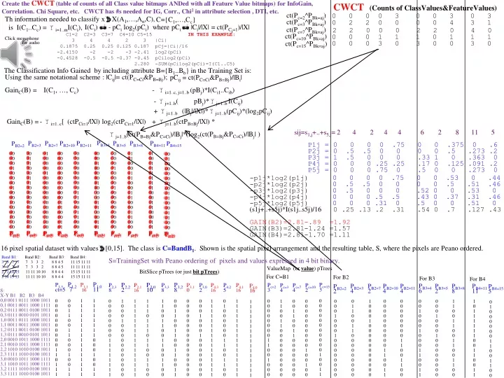
Create the CWCT (table of counts of all Class value bitmaps ANDed with all Feature Value bitmaps) for InfoGain, Correlation. Chi Square, etc. CWCT has #s needed for IG, Corr., Chi2 in attribute selection , DTI, etc. S1,j= 0 0 0 0 3 0 0 3 0 3 ct(Pc=2^PBk=aj) CWCT (Counts of ClassValues&FeatureValues) S2,j= 0 2 2 0 0 0 0 4 3 1 ct(Pc=3^PBk=aj) Th information needed to classify xX(A1,…,An,C), is I(C1..Cc) = i=1..mI(Ci), C={C1,…,Cc} S3,j= 2 2 0 0 0 2 2 0 4 0 ct(Pc=7^PBk=aj) I(Ci) - pCi log2(pCi) where pCi |Ci|/|X| = ct(PCi=1)/|X| S4,j= 0 0 0 1 1 1 0 1 1 1 ct(Pc=10^PBk=aj) 0 0 0 0 0 0 0 0 1 1 0 0 1 0 0 0 0 0 0 0 0 0 0 0 1 1 0 0 1 0 0 0 0 0 0 0 0 0 0 0 1 1 0 0 1 0 0 0 0 0 0 0 0 0 0 0 1 1 0 0 1 0 0 0 0 0 0 0 0 0 0 0 1 1 0 0 1 0 0 0 0 0 0 0 0 0 0 0 1 1 0 0 1 0 0 0 0 0 0 0 0 0 0 0 1 1 0 0 1 0 0 0 0 0 0 0 0 0 0 0 1 1 0 0 1 0 0 0 0 0 0 0 0 0 0 0 1 1 0 0 1 0 0 0 0 0 0 0 0 0 0 0 1 1 0 0 1 0 0 0 S5,j= 0 0 0 3 0 3 0 0 3 0 ct(Pc=15^PBk=aj) C1=2 C2=3 C3=7 C4=10 C5=15 IN THIS EXAMPLE: 3 4 4 2 3 |Ci| 0.1875 0.25 0.25 0.125 0.187 pCj=|Ci|/16 -2.4150 -2 -2 -3 -2.41 log2(pCi) -0.4528 -0.5 -0.5 -0.37 -0.45 pCilog2(pCi) 2.280 -SUM(pCilog2(pCi)=I(C1..C5) Click megaphone for audio sij=s1,j+..+s5,j= 2 4 2 4 4 6 2 8 115 The Classification Info Gained by including attribute B={B1..Bb} in the Training Set is: P1j = 0 0 0 0 .75 0 0 .375 0 .6 P2j = 0 .5 .5 0 0 0 0 .5 .273 .2 P3j = 1 .5 0 0 0 .33 1 0 .363 0 P4j = 0 0 0 .25 .25 .17 0 .125 .091 .2 P5j = 0 0 0 .75 0 .5 0 0 .273 0 Using the same notational scheme : |Cij|= ct(PC=Ci&PB=Bj); pCij = ct(PC=Ci&PB=Bj)/|Bi| GainC(B) = I(C1, …, Cc) - i=1..c, j=1..b (pBj)*I(Ci1..Cib) 0 0 0 0 0 0 0 0 0 0 0 1 0 0 1 1 0 0 0 0 0 0 0 0 0 0 0 1 0 0 1 1 0 0 0 0 0 0 0 0 0 0 0 1 0 0 1 1 0 0 0 0 0 0 0 0 0 0 0 1 0 0 1 1 0 0 0 0 0 0 0 0 0 0 0 1 0 0 1 1 0 0 0 0 0 0 0 0 0 0 0 1 0 0 1 1 0 0 0 0 0 0 0 0 0 0 0 1 0 0 1 1 0 0 0 0 0 0 0 0 0 0 0 1 0 0 1 1 0 0 0 0 0 0 0 0 0 0 0 1 0 0 1 1 0 0 0 0 0 0 0 0 0 0 0 1 0 0 1 1 0 0 1 1 0 0 1 1 0 0 0 0 0 0 0 0 0 0 1 1 0 0 1 1 0 0 0 0 0 0 0 0 0 0 1 1 0 0 1 1 0 0 0 0 0 0 0 0 0 0 1 1 0 0 1 1 0 0 0 0 0 0 0 0 0 0 1 1 0 0 1 1 0 0 0 0 0 0 0 0 0 0 1 1 0 0 1 1 0 0 0 0 0 0 0 0 0 0 1 1 0 0 1 1 0 0 0 0 0 0 0 0 0 0 1 1 0 0 1 1 0 0 0 0 0 0 0 0 0 0 1 1 0 0 1 1 0 0 0 0 0 0 0 0 0 0 1 1 0 0 1 1 0 0 0 0 0 0 0 0 1 1 0 0 1 1 0 0 0 0 0 0 0 0 0 0 1 1 0 0 1 1 0 0 0 0 0 0 0 0 0 0 1 1 0 0 1 1 0 0 0 0 0 0 0 0 0 0 1 1 0 0 1 1 0 0 0 0 0 0 0 0 0 0 1 1 0 0 1 1 0 0 0 0 0 0 0 0 0 0 1 1 0 0 1 1 0 0 0 0 0 0 0 0 0 0 1 1 0 0 1 1 0 0 0 0 0 0 0 0 0 0 1 1 0 0 1 1 0 0 0 0 0 0 0 0 0 0 1 1 0 0 1 1 0 0 0 0 0 0 0 0 0 0 1 1 0 0 1 1 0 0 0 0 0 0 0 0 0 0 0 0 0 0 0 0 0 0 0 0 1 0 0 1 0 0 0 0 0 0 0 0 0 0 0 0 1 0 0 1 0 0 0 0 0 0 0 0 0 0 0 0 1 0 0 1 0 0 0 0 0 0 0 0 0 0 0 0 1 0 0 1 0 0 0 0 0 0 0 0 0 0 0 0 1 0 0 1 0 0 0 0 0 0 0 0 0 0 0 0 1 0 0 1 0 0 0 0 0 0 0 0 0 0 0 0 1 0 0 1 0 0 0 0 0 0 0 0 0 0 0 0 1 0 0 1 0 0 0 0 0 0 0 0 0 0 0 0 1 0 0 1 0 0 0 0 0 0 0 0 0 0 0 0 1 0 0 1 0 0 - j=1..b( pBj)*j=1..b I(Cij) 0 0 0 0 .75 0 0 .53 0 .44 0 .5 .5 0 0 0 0 .5 .51 .46 0 .5 0 0 0 .52 0 0 .53 0 0 0 0 .5 .5 .43 0 .37 .31 .46 0 0 0 .31 0 .5 0 0 .51 0 -p1j*log2(p1j) -p2j*log2(p2j) -p3j*log2(p3j) -p4j*log2(p4j) -p5j*log2(p5j) (s1j+..+s5j)*I(s1j..s5j)/16 0 .25 .13 .2 .31 .54 0 .7 .127 .43 GAIN(B2)=2.81-.89 =1.92 GAIN(B3)=2.81-1.24 =1.57 GAIN(B4)=2.81-1.70 =1.11 Pc=2 Pc=2 Pc=2 Pc=2 Pc=2 Pc=2 Pc=2 Pc=2 Pc=2 Pc=2 + j=1..b (|Bj|/|X|)*j=1..b(pCij)*(log2pCij) - i=1..c[ (ctPCi=1/|X|) log2(ctPCi=1/|X|) GainC(B) = + j=1..b(ctPB=Bj/|X|) * ct(PB=Bj&PC=Ci)/|Bj| ) j=1..b(ct(PB=Bj&PC=Ci)/|Bj|*(log2( P3,3 8 P1,2 7 P2,1 16 P3,2 8 P2,0 10 P3,0 2 P2,3 8 P4,1 16 P2,2 2 P1,3 ct=5 P3,1 0 Pc=7 4 P4,2 5 P1,1 16 P1,0 11 Pc=3 4 P4,0 16 P4,3 16 Pc=10 2 Pc=15 3 Pc=2 3 Pc=15 Pc=15 Pc=15 Pc=15 Pc=15 Pc=15 Pc=15 Pc=15 Pc=15 Pc=15 Pc=7 Pc=7 Pc=7 Pc=7 Pc=7 Pc=7 Pc=7 Pc=7 Pc=7 Pc=7 Pc=3 Pc=3 Pc=3 Pc=3 Pc=3 Pc=3 Pc=3 Pc=3 Pc=3 Pc=3 Pc=10 Pc=10 Pc=10 Pc=10 Pc=10 Pc=10 Pc=10 Pc=10 Pc=10 Pc=10 0 0 0 0 0 0 0 0 1 1 0 0 1 0 0 0 1 1 1 1 1 1 1 1 1 1 1 1 1 1 1 1 0 1 0 0 0 0 0 0 1 1 0 0 1 1 0 0 1 0 0 0 1 0 0 0 0 0 0 0 0 0 0 0 1 1 1 1 1 1 1 1 1 1 1 1 1 1 1 1 0 0 0 1 0 0 0 1 0 0 0 0 0 0 0 0 0 0 0 0 0 0 0 0 1 1 1 1 1 1 1 1 1 1 0 0 1 1 0 0 1 1 0 0 1 1 0 0 1 1 1 1 1 1 1 1 1 1 1 1 1 1 1 1 0 0 1 1 0 0 1 1 0 0 1 1 0 0 1 1 0 0 0 0 0 0 0 0 0 0 0 1 0 0 1 1 1 1 1 1 1 1 1 1 1 1 1 1 1 1 1 1 0000000000110111 1 1 1 1 1 1 1 1 0 0 0 1 0 0 1 1 1 1 0 0 1 1 0 0 0 0 0 0 0 0 0 0 1 1 1 1 1 1 1 1 1 1 1 1 1 1 1 1 0 0 0 0 0 0 0 0 0 0 0 0 0 0 0 0 0 0 0 0 0 0 0 0 0 0 1 0 0 1 0 0 1 1 1 0 1 1 1 0 1 1 0 0 1 1 0 0 0 0 1 1 0 0 1 1 0 0 0 0 0 0 0 0 0 0 1 1 0 0 1 1 0 0 0 1 0 0 1 1 16 pixel spatial dataset with values[0,15]. The class is C=BandB1. Shown is the spatial pixel arrangement and the resulting table, S, where the pixels are Peano ordered. Band B1: Band B2: Band B3: Band B4: 3 3 7 7 7 3 3 2 8 8 4 5 11 15 11 11 3 3 7 7 7 3 3 2 8 8 4 5 11 11 11 11 2 2 10 15 11 11 10 10 8 8 4 4 15 15 11 11 2 10 15 15 11 11 10 10 8 8 4 4 15 15 11 11 S=TrainingSet with Peano ordering of pixels and values expressed in 4 bit binary. ValueMap (or value) pTrees BitSlice pTrees (or just bit pTrees) For C=B1 For B2 For B3 For B4 PB3=4 PB3=4 6 PB2=3 4 PB2=3 PB2=7 2 PB2=7 PB2=10 PB2=10 4 PB2=11 PB2=11 4 PB3=5 PB3=5 2 PB3=8 8 PB3=8 PB4=11 11 PB4=11 PB4=15 PB4=15 5 PB2=2 PB2=2 2 S: X-Y B1 B2 B3 B4 0,0 0011 0111 1000 1011 0,1 0011 0011 1000 1111 0,2 0111 0011 0100 1011 0,3 0111 0010 0101 1011 1,0 0011 0111 1000 1011 1,1 0011 0011 1000 1011 1,2 0111 0011 0100 1011 1,3 0111 0010 0101 1011 2,0 0010 1011 1000 1111 2,1 0010 1011 1000 1111 2,2 1010 1010 0100 1011 2,3 1111 1010 0100 1011 3,0 0010 1011 1000 1111 3,1 1010 1011 1000 1111 3,2 1111 1010 0100 1011 3,3 1111 1010 0100 1011 0 0 0 1 0 0 0 1 0 0 0 0 0 0 0 0 0 0 0 1 0 0 0 1 0 0 0 0 0 0 0 0 0 1 1 0 0 1 1 0 0 0 0 0 0 0 0 0 0 1 1 0 0 1 1 0 0 0 0 0 0 0 0 0 1 0 0 0 1 0 0 0 0 0 0 0 0 0 0 0 1 0 0 0 1 0 0 0 0 0 0 0 0 0 0 0 0 0 0 0 0 0 0 0 0 0 1 1 0 0 1 1 0 0 0 0 0 0 0 0 0 0 1 1 0 0 1 1 0 0 0 0 0 0 0 0 1 1 0 0 1 1 0 0 0 0 0 0 0 0 0 0 1 1 0 0 1 1 0 0 0 0 1 0 0 0 1 0 0 0 1 1 0 0 1 1 0 0 1 0 0 0 1 0 0 0 1 1 0 0 1 1 0 0 0 1 0 0 0 1 0 0 0 0 0 0 0 0 0 0 0 1 0 0 0 1 0 0 0 0 0 0 0 0 1 1 0 0 1 1 0 0 1 1 0 0 1 1 0 0 1 1 0 0 1 1 0 0 1 1 0 0 1 1 0 0 1 0 1 1 1 1 1 1 0 0 1 1 0 0 1 1 1 0 1 1 1 1 1 1 0 0 1 1 0 0 1 1 0 1 0 0 0 0 0 0 1 1 0 0 1 1 0 0 0 1 0 0 0 0 0 0 1 1 0 0 1 1 0 0
ClassWise Counts: Always use Class Order in every Classification TrainingSet X=(B1,B2,B3.B4). Let the class be B2. The ordering of a RSI table is usually a spatial pixel ordering (e.g., raster, Penao (Z), or Hilbert) Here we detail the advantage of ordering by class instead. In fact, we recommend sorting every classification training set by class, before converting to pTrees. 1. Order the TrainingSet by Class (using a rough bucket sort?) . 2. Create all value pTrees for allo feature attribute, B1, B3 and B4. 3. Create CWCT (ClassWiseCountTable) of countt(PC=ci&PB=Bj) j=1,3,4, by applying CWC(PB=Bj) (ClassWiseCount operator) to each feature value bitmap Band4 11 15 11 11 11 11 11 11 15 15 11 11 15 15 11 11 Band1 3 3 7 7 3 3 7 7 2 2 10 15 2 10 15 15 Band2=Class 7 3 3 2 7 3 3 2 11 11 10 10 11 11 10 10 Band3 8 8 4 5 8 8 4 5 8 8 4 4 8 8 4 4 So the only operation is to apply to each feature value pTree, the ClassWiseCount operation. It can be applied in parallel to all feature value pTrees concurrently (on a “pTreeSet replicated” cluster) Thus, time to compute and compare (to threshold ) all Col InfoGains, is approx. time cost of one CWC So, it is paramount to fully optimize the code for the CWC operation! Substituting Pearson Correlation or Chi Square for Info Gain, CFC is all that’s needed. Important point: We never computed pairwise ANDS of class value and feature value pTrees, because we ‘ve bucket sorted the TrainingSet by class (a fast sort) before creating our value pTrees. And, again, once the CWC operator has created the table of class OneCounts for each feature column (e.g., below) the rest of the InfoGain (or Correlation or Chi Square) calculation is scalar arithmetic. Alternatively, use “Variable Length Stride” Multilevel pTrees, where leaf stride lengths are class sizes. For this Classification TrainingSet, we’d use 2-level pTrees with 5 leaf stride of lengths, 2,4,2,4,4 resp: 1. Rough [bucket] sort by class C=B1 Peano Ordered Training TableB1-vmaps B3-vmaps B4-vmaps x,y rrn CL=B2 B1 237af B3 458 B4 bf 0,0 0 7 3 01000 8 001 11 10 0,1 1 3 3 01000 8 001 15 01 1,0 2 7 3 01000 8 001 11 10 1,1 3 3 3 01000 8 001 11 10 0,2 4 3 7 00100 4 100 11 10 0,3 5 2 7 00100 5 010 11 10 1,2 6 3 7 00100 4 100 11 10 1,3 7 2 7 00100 5 010 11 10 2,0 8 11 2 10000 8 001 15 01 2,1 9 11 2 10000 8 001 15 01 3,0 a 11 2 10000 8 001 15 01 3,1 b 11 10 00010 8 001 15 01 2,2 c 10 10 00010 4 100 11 10 2,3 d 10 15 00001 4 100 11 10 X.Class.16:2,4,2,4,4.PB4=f 3,2 e 10 15 00001 4 100 11 10 3,3 f 10 15 00001 4 100 11 10 5:0,1,0,0,4 Terminology: “Class” pTree (ordered by class. List the variable stride lengths in the name. Included in the root node (since not used for anything else) total Count of full pTree followed by the 5 class counts. This should all be pre-computed and store with the pTree(then our table can be read off the root of the pTree). 1000 00 1111 00 0000 Next slides we will give more justification for the pTree rule: CW Rule: Always order any Classification Training Set by Class!(then convert to pTrees). I.e., Training Sets should always be Class Ordered!!! Click megaphones for audio CWC(PB1=7,2,6,8,c) CWC(PB1=a,2,6,8,c) etc... 3. Apply ClassWiseCount to each feature attribute Value Map pTree CWC(P,ClassOffsetList) CWC(PB4=f,2,6,8,c) etc. CWC(PB1=2,2,6,8,c) ClassStartOffsets CWC(PB1=3,2,6,8,c) • Create value pTrees for feature attributes • B1, B3, B4 X (after Class sort)B1vpTrees B3-vpTrees B4-vpTrees x,y rrn class B1 237af B3 458 B4 bf P1=f P1=2 P4=b P1=3 P1=7 P1=a P3=4 P4=f P3=5 P3=8 C= 2 bucket 0 2 0 2 0 0 1 2 3 4 5 6 7 8 9 a b c d e f 0 0 2 0 0 C= 3 bucket 0 3 2 0 2 0 2 2 0 1 C= 7 bucket 0 2 0 0 2 0 2 0 0 0 C=10 bucket 3 4 4 0 0 0 0 0 1 0 C=11 bucket 0 0 0 1 4 3 0 0 1 4 CWCT: ClassValue&FeatureVaue Count table
SCW: Secure Classwise technology 1 2 3 4 5 6 7 8 9 0 1 2 3 4 5 6 7 8 9 0 FOG Similar to the cloud, but can see only a few feet (only your authorized pTrees . Use with Id Fusion to solve Snowden problem? RSI1_16 Band1 3 3 7 7 3 3 7 7 2 2 10 15 2 10 15 15 1 2 3 4 5 Band4 11 15 11 11 11 11 11 11 15 15 11 11 15 15 11 11 Band2=Class 7 3 3 2 7 3 3 2 11 11 10 10 11 11 10 10 Band3 8 8 4 5 8 8 4 5 8 8 4 4 8 8 4 4 0 1 2 3 4 5 6 7 8 9 0 1 2 3 4 5 6 7 8 9 0 1 2 3 4 5 6 7 8 9 0 1 2 3 4 5 6 7 8 9 0 1 2 3 4 5 6 7 8 9 0 1 0 0 0 0 0 0 0 0 0 1 1 1 0 0 0 1 1 1 0 0 0 0 0 0 0 0 0 0 0 0 0 0 1 1 1 1 1 1 1 1 1 1 1 1 1 1 1 1 0 1 2 3 4 5 6 7 8 9 0 0 0 1 1 1 1 0 0 0 0 0 0 0 0 0 0 1 1 1 1 1 1 1 1 1 1 1 1 1 1 1 1 0 0 0 0 0 0 1 1 0 0 0 0 0 0 0 0 0 0 1 1 0 0 1 1 0 0 0 0 0 0 0 0 0 0 0 0 0 0 0 0 0 0 0 0 1 1 1 1 0 1 2 3 4 5 6 7 8 9 0 1 1 0 1 1 1 1 1 1 1 1 1 0 0 0 0 0 0 0 0 0 0 0 0 1 1 1 0 0 0 0 0 0 0 0 0 0 0 0 0 0 0 0 0 1 1 1 1 0 0 0 0 0 0 0 0 1 0 0 0 0 0 0 1 0 1 2 3 4 5 6 7 8 9 0 0 0 0 0 0 0 1 1 0 0 0 0 0 0 0 0 0 0 1 0 0 0 0 0 0 0 0 0 1 1 1 1 0 1 2 3 4 5 6 7 8 9 0 1 1 0 0 1 1 0 0 1 1 1 1 0 0 0 0 0 0 0 0 0 0 0 0 0 0 0 0 0 0 0 0 TOC ct cls-ct’s FOG relative pTree number RSI1._16(24244).Offset rpn FOG Offset column is the key for authorized users. Authorization by band=column? Store separately by pTree and class so authorization can be restricted to feature col and class Another security layer would pre-pend to each pTree a random length pad, Add-A-Pad. This is shown on the next slide. Is it necessary? Is it useful?? Then there’d be 2 keys, the FOG.offset sequence and PAD.length sequence. 1 1 0 0 0 0 0 0 0 0 0 0 0 0 0 0 1 1 1 1 1 1 1 1 1 1 1 1 1 1 1 1 P1,3.4(00031).3402 0 P1,2.6(02040).1934 1 0 1 2 3 4 5 6 7 8 9 0 P1,1.e(24234).4981 2 1 1 1 1 1 1 1 1 1 1 1 1 0 0 0 0 P1,0.a(24240).0045 3 P1=2.3(00030).2219 4 P1=3.4(02200).5011 5 0 0 1 1 1 1 1 1 0 0 0 0 1 1 1 1 P1=7.4(22000).2480 6 P1=a.2(00011).0023 7 0 1 2 3 4 5 6 7 8 9 0 P1=f.3(00030).4056 8 0 0 0 0 0 0 0 0 1 1 1 1 0 0 0 0 0 0 0 0 0 0 0 0 0 1 1 1 0 0 0 0 0 0 1 1 0 0 1 1 0 0 0 0 1 1 1 1 P2,3.8(00044).4683 9 P2,2.g(00200).1710 10 P2,1.g(24244).1781 11 0 1 2 3 4 5 6 7 8 9 0 P2,0.a(04204).0750 12 P2=2.2(20000).1102 13 P2=3.4(04000).2609 14 P2=7.2(00200).0629 15 P2=a.4(00040).5155 16 P2=f.4(00004).3822 17 0 1 2 3 4 5 6 7 8 9 0 1 1 0 0 1 1 0 0 1 1 1 1 0 0 0 0 P3,3.8(02204).1556 18 P3,2.8(22040).2975 19 0 0 0 0 1 1 0 0 1 1 1 1 0 0 0 0 P3,1.0(00000).1034 20 1 1 0 0 1 1 0 0 0 0 0 0 0 0 0 0 1 1 0 0 0 0 0 0 0 0 0 0 0 0 0 0 P2,0.2(20000).4440 21 1 1 1 1 1 1 1 1 1 1 1 1 1 1 1 1 1 1 1 1 1 1 1 10 1 1 1 1 1 1 1 P3=4.6(02040).3377 22 0 0 1 0 0 0 0 0 0 0 0 0 1 1 1 1 0 1 2 3 4 5 6 7 8 9 0 00 0 0 0 0 0 1 1 1 1 1 1 1 1 0 0 1 1 0 0 1 1 0 0 0 0 1 1 1 1 P3=5.2(20000).3480 23 P3=8.8(02204).0784 24 P4,3.g(24244).4510 25 P4,2.6(01004).2583 26 P4,1.e(24244).2740 27 The CWCT (Class&Feature Count Table) is available in TOC. P4,0.g(24244).0503 28 P4=b.b(23240).3218 29 P4=f .5(01004).3430 30
NO! SCW-A with Add-A-Pad? 1 2 3 4 5 6 7 8 9 0 1 2 3 4 5 6 7 8 9 0 The FOG (Similar to cloud, but can see only a few feet (your authorized pTrees ), AKA pTreesoup 1 2 3 4 5 0 1 2 3 4 5 6 7 8 9 0 1 2 3 4 5 6 7 8 9 0 1 2 3 4 5 6 7 8 9 0 1 2 3 4 5 6 7 8 9 0 1 2 3 4 5 6 7 8 9 0 1 RSI1_16 Band1 3 3 7 7 3 3 7 7 2 2 10 15 2 10 15 15 Band4 11 15 11 11 11 11 11 11 15 15 11 11 15 15 11 11 Band2=Class 7 3 3 2 7 3 3 2 11 11 10 10 11 11 10 10 Band3 8 8 4 5 8 8 4 5 8 8 4 4 8 8 4 4 0 10 0 0 0 0 0 0 0 0 1 1 1 0 0 0 1 0 1 1 0 0 0 0 0 0 0 0 0 0 0 0 0 0 1 1 1 1 1 1 1 1 1 1 1 1 1 1 1 1 0 1 2 3 4 5 6 7 8 9 0 1 0 0 1 1 1 1 0 0 0 0 0 0 0 0 0 0 0 0 0 1 1 1 1 1 1 1 1 1 1 1 1 1 1 1 1 101 0 0 0 0 0 0 1 1 0 0 0 0 0 0 0 0 1 0 0 1 1 0 0 1 1 0 0 0 0 0 0 0 0 0 1 2 3 4 5 6 7 8 9 0 0 0 0 0 0 0 0 0 0 0 0 0 1 1 1 1 0 1 1 1 0 1 1 1 1 1 1 1 1 1 0 0 0 0 10 0 0 0 0 0 0 0 0 1 1 1 0 0 0 0 0 0 0 0 0 0 0 0 0 0 0 0 0 0 0 0 1 1 1 1 00 0 0 0 0 0 0 0 0 1 0 0 0 0 0 0 1 0 1 2 3 4 5 6 7 8 9 0 1 1 0 0 0 0 0 0 1 1 0 0 0 0 0 0 0 0 0 0 1 0 0 0 0 0 0 0 0 0 1 1 1 1 0 1 2 3 4 5 6 7 8 9 0 1 1 0 0 1 1 0 0 1 1 1 1 0 0 0 0 1 1 0 0 0 0 0 0 0 0 0 0 0 0 0 0 0 0 TOC Ct ClassCt FOG PAD length RSI1._16(24244).offset rpn pl 1 1 0 0 0 0 0 0 0 0 0 0 0 0 0 0 0 1 1 1 1 1 1 1 1 1 1 1 1 1 1 1 1 P1,3.4(00031).3402 0 2 P1,2.6(02040).1934 1 0 AAP: Add-A-Pad security layer Pre-pend to each pTree a random length pad. Useful? There are 2 keys: FOG offset array, PAD.length array. Add-A-Pad strengthen security? Or do random background bits already do what AAP does? I.e., Iff you know both keys, you have pTree start offsets. I’m going to assume AAP does not enhance security, so I ‘ll go back to the previous slide where the FOG offset array is the key. CWCT is available in the TOC 0 1 2 3 4 5 6 7 8 9 0 P1,1.e(24234).4981 2 3 00 1 1 1 1 1 1 1 1 1 1 1 1 0 0 0 0 P1,0.a(24240).0045 3 2 P1=2.3(00030).2219 4 2 2 P1=3.4(02200).5011 5 1 0 0 1 1 1 1 1 1 0 0 0 0 1 1 1 1 P1=7.4(22000).2480 6 1 P1=a.2(00011).0023 7 2 0 1 2 3 4 5 6 7 8 9 0 P1=f.3(00030).4056 8 0 0 0 0 0 0 0 0 0 1 1 1 1 0 0 0 0 0 0 0 0 0 0 0 0 0 1 1 1 0 0 0 0 0 0 1 1 0 0 1 1 0 0 0 0 1 1 1 1 P2,3.8(00044).4683 9 0 P2,2.g(00200).1710 10 3 P2,1.g(24244).1781 11 1 0 1 2 3 4 5 6 7 8 9 0 P2,0.a(04204).0750 12 0 P2=2.2(20000).1102 13 1 P2=3.4(04000).2609 14 1 P2=7.2(00200).0629 15 2 P2=a.4(00040).5155 16 0 P2=f.4(00004).3822 17 3 0 1 2 3 4 5 6 7 8 9 0 0 1 1 0 0 1 1 0 0 1 1 1 1 0 0 0 0 P3,3.8(02204).1556 18 0 P3,2.8(22040).2975 19 1 0 0 0 0 0 1 1 0 0 1 1 1 1 0 0 0 0 P3,1.0(00000).1034 20 2 0 1 1 0 0 1 1 0 0 0 0 0 0 0 0 0 0 1 0 1 1 0 0 0 0 0 0 0 0 0 0 0 0 0 0 P2,0.2(20000).4440 21 0 1 1 1 1 1 1 1 1 1 1 1 1 1 1 1 1 1 0 1 11 1 1 1 1 1 1 10 1 1 1 1 1 1 1 P3=4.6(02040).3377 22 1 0 0 1 0 0 0 0 0 0 0 0 0 1 1 1 1 0 1 2 3 4 5 6 7 8 9 0 00 0 0 0 0 0 1 1 1 1 1 1 1 1 0 0 1 1 0 0 1 1 0 0 0 0 1 1 1 1 P3=5.2(20000).3480 23 2 P3=8.8(02204).0784 24 0 P4,3.g(24244).4510 25 3 P4,2.6(01004).2583 26 0 P4,1.e(24244).2740 27 1 P4,0.g(24244).0503 28 0 P4=b.b(23240).3218 29 2 P4=f .5(01004).3430 30 0
SCW-M: Secure ClassWise Multilevel pTrees 1 2 3 4 5 6 7 8 9 0 1 2 3 4 5 6 7 8 9 0 SCOM pTree FOGLike a cloud but one can see only a few feet (only your authorized pTrees A really exciting thesis topic would be to develop this with the so-called Bell Lapadula Model of Multilevel Security in the US Defense Department Orange Book!!!! (Easily modified to fit the Bell Lapadula Model?) Columns (+rows) can have different security levels, which is what Bell-Lapadula is all about. In traditional horizontal DBs that is hard to implement. It seems easier using SCOM. 1 2 3 4 5 0 1 2 3 4 5 6 7 8 9 0 1 2 3 4 5 6 7 8 9 0 1 2 3 4 5 6 7 8 9 0 1 2 3 4 5 6 7 8 9 0 1 2 3 4 5 6 7 8 9 0 1 1 1 1 1 1 1 0 0 0 0 0 0 0 0 0 0 0 0 1 1 0 0 0 0 1 1 0 1 2 3 4 5 6 7 8 9 0 0 0 0 0 0 0 0 0 0 0 0 0 0 0 0 0 0 0 0 0 0 0 0 0 0 0 TOC Ct Cls Strides (PRE-COMPUTE THIS!) RSI1._16(24244) C1 C2 C3 C4 C5<- Class 1 1 1 1 1 1 0 0 0 0 0 0 0 0 1 1 0 0 0 0 0 0 0 0 0 0 P1,3.4(00031).3402.3206.1706.2060.4040 <-pTree offsets 0 1 2 3 4 5 6 7 8 9 0 0 0 0 0 P1,2.6(02040).1934.0520.2050.4568.2966 0 0 0 0 0 0 0 0 P1,1.e(24234).4981.5080.5171.2450.4940 1 1 0 1 1 1 P1,0.a(24240).0045.2530.0060.1540.3561 0 0 0 0 0 1 1 1 0 0 0 1 0 0 1 1 0 0 0 0 P1=2.3(00030).2219.2306.3906.1629.3980 0 0 P1=3.4(02200).5011.4530.4538.4604.0070 0 0 0 1 2 3 4 5 6 7 8 9 0 P1=7.4(22000).2480.3050.2460.1077.2871 P1=a.2(00011).0023.0010.1120.0430.0420 0 0 0 0 P1=f.3(00030).4056.5036.5128.5119.5047 0 0 0 0 0 0 0 0 1 1 1 0 0 0 0 0 1 0 0 0 1 1 0 0 1 1 1 1 0 0 P2,3.8(00044).4683.4590.4690.4071.5090 P2,2.g(00200).1710.1502.1900.2601.2906 0 1 2 3 4 5 6 7 8 9 0 1 1 P2,1.g(24244).1781.2080.0098.0080.0470 0 0 P2,0.a(04204).0750.0450.0558.0051.0145 0 0 0 0 0 0 0 0 0 0 0 0 1 1 P2=2.2(20000).1102.1406.1401.1916.2017 0 0 0 1 1 1 1 1 1 1 1 1 1 1 P2=3.4(04000).2609.3009.3510.2310.2325 1 1 P2=7.2(00200).0629.0001.0310.0321.0336 P2=a.4(00040).5155.3547.3568.0369.0090 0 1 2 3 4 5 6 7 8 9 0 P2=f.4(00004).3822.3925.3930.4010.4000 1 1 1 1 1 1 0 0 0 0 0 0 0 0 P3,3.8(02204).1556.0450.1060.1963.2065 P3,2.8(22040).2975.3077.2570.1065.0636 0 0 0 1 1 1 1 1 1 1 0 0 1 1 0 0 0 0 0 0 P3,1.0(00000).1034.0636.1034.0636.0636 P2,0.2(20000).4440.1120.1034.0636.0636 0 1 2 3 4 5 6 7 8 9 0 0 0 P3=4.6(02040).3377.3187.3170.0476.0580 0 0 0 0 P3=5.2(20000).3480.0001.0023.0001.0001 1 1 P3=8.8(02204).0784.0189.1089.0988.1580 1 1 0 1 1 1 1 1 0 0 1 1 0 0 0 0 0 0 1 1 1 1 P4,3.g(24244).4510.0145.0045.0145.0145 0 0 0 0 0 1 2 3 4 5 6 7 8 9 0 P4,2.6(01004).2583.2686.2588.2990.2980 1 1 1 1 1 1 1 1 0 0 0 0 P4,1.e(24244).2740.0145.0160.0145.0145 1 1 1 1 P4,0.g(24244).0503.0145.0160.0145.0145 0 0 1 1 1 1 0 0 0 0 0 0 0 0 1 1 1 1 P4=b.b(23240).3218.2920.0045.0080.0001 0 0 0 0 1 1 P4=f .5(01004).3430.2686.0023.0010.0369 0 1 2 3 4 5 6 7 8 9 0 The CWCT is available in the TOC. 1 1 1 1 1 1 0 0 0 0 0 0 0 0 1 1 Bell Lapadula says a user can read down and write up with respect to the security hierarchy. Suppose Feature Columns 3,4 are secret 1 is confidential and in 2 (class column) C1,C2 are unclassified , C3 is confidential and C4,C5 are secret. Then a Confidential user would be given as a read key: 0 0 0 0 1 1 1 1 1 1 1 1 1 1 1 1 1 1 1 1 1 1 0 0 0 0 1 1 1 1 1 1 1 1 0 0 0 1 2 3 4 5 6 7 8 9 0 0 0 0 1 0 0 0 0 0 1 1 0 0 0 0 0 0 1 1 0 0 1 1 0 0 0 0 0 0 0 0 0 0 1 1 1 1 0 0 0 0 How big is a big data spatial data set these days? Cover a forest with 10K gridded ultrahi res images (3840x2160) 8.29B pixels At 1 micrsec/pixel, VPHD takes 8,294sec=2.3 hrs. 1 1
RSI-2 C=B1, ClassOrdered Band2=Green 7 3 3 2 7 3 3 2 11 11 10 10 11 11 10 10 Band5=NIR: 2 2 7 7 2 2 7 7 2 2 15 15 2 15 15 15 Band3=Red 8 8 4 5 8 8 4 5 8 8 4 4 8 8 4 4 Band4=Blue 11 15 11 11 11 11 11 11 15 15 11 11 15 15 11 11 Band6=MIR 11 11 11 11 11 11 11 11 15 15 11 11 15 15 11 11 Band7=FIR: 8 8 4 5 8 8 4 5 8 8 8 8 8 8 8 8 Band8=TIR 2 3 7 7 3 3 7 7 2 2 15 15 2 15 15 15 Band1=Yield 3 3 7 7 3 3 7 7 2 2 10 15 2 10 15 15 Band9=UV2 15 15 15 15 15 15 15 15 2 2 15 15 2 15 15 15 Bandd=UVd 0 0 0 0 0 0 0 0 0 0 0 15 0 0 15 15 Banda=UVa: 3 3 15 15 3 3 15 15 15 15 15 15 15 15 15 15 Bandb=UVb 15 15 7 7 15 15 7 7 15 15 15 15 15 15 15 15 Bandc=UVc 0 0 0 0 0 0 0 0 0 0 10 0 0 10 0 0 CWCT: ClassWise Count Table (Class-value & Feature-value Count table) Feature Band#-> 1 1 1 1 1 2 2 2 2 2 3 3 3 4 4 5 5 5 6 6 Feature Value-> 2 3 7 a f 2 3 7 a b 4 5 8 b f 2 7 f b f Class: C=3 0 4 0 0 0 0 2 2 0 0 0 0 4 3 1 4 0 0 4 0 C=7 0 0 4 0 0 1 2 0 0 0 2 2 0 4 0 0 4 0 4 0 C=2 3 0 0 0 0 0 0 0 0 3 0 0 3 0 3 3 0 0 0 3 C=10 0 0 0 2 0 0 0 0 1 1 1 0 1 1 1 0 0 2 1 1 C=15 0 0 0 0 3 0 0 0 3 0 3 0 0 3 0 0 0 3 3 0 P1=15 3 P2=11 4 P1=2 3 P2=2 2 P1=3 4 P1=7 4 P1=10 2 P2=3 4 P2=7 2 P2=10 4 P1,3 5 P1,2 7 P1,1 16 P1,0 11 P2,3 8 P2,2 2 P2,1 16 P2,0 10 P4,3 16 P4,2 5 P4,1 16 P5=15 5 P5,3 5 P5,2 9 P5,1 16 P5,0 9 P3,2 10 P3,1 6 P3,0 2 P5=2 7 P4,0 16 P5=7 4 P6,3 16 P6,2 4 P3=4 6 P3=5 2 P3=8 8 P4=11 11 P4=15 5 P6,1 16 P6=15 4 P6,0 16 P6=11 12 7 3 7 3 3 2 3 2 11 11 11 11 10 10 10 10 B2 =G 8 8 8 8 4 5 4 5 8 8 8 8 4 4 4 4 B3 =R 11 15 11 11 11 11 11 11 15 15 15 15 11 11 11 11 B4 =B 1 1 1 1 0 0 0 0 0 0 0 0 0 0 0 0 0 0 0 0 1 1 1 1 0 0 0 0 0 0 0 0 0 0 0 0 0 0 0 0 0 0 0 1 1 0 0 0 0 1 0 1 1 0 1 0 0 0 0 0 0 0 0 0 1 0 1 0 0 0 0 0 0 0 0 0 0 0 0 0 0 0 0 0 0 0 0 0 0 0 0 0 1 1 1 1 0 0 0 0 0 1 0 1 0 0 0 0 0 0 0 0 1 1 1 1 0 0 0 0 1 1 1 1 0 0 0 0 3 3 3 3 7 7 7 7 2 2 2 10 10 15 15 15 B1 =Y 0000000000011111 0 0 0 0 1 1 1 1 0 0 0 0 0 1 1 1 1 1 1 1 1 1 1 1 1 1 1 1 1 1 1 1 1 1 1 1 1 1 1 1 0 0 0 0 0 1 1 1 0 0 0 0 0 0 0 0 0 0 0 0 0 1 1 1 0000000011111111 1 0 1 0 0 0 0 0 0 0 0 0 0 0 0 0 1 1 1 1 1 1 1 1 1 1 1 1 1 1 1 1 1 1 1 1 1 0 1 0 1 1 1 1 0 0 0 0 0 0 0 0 0 0 0 0 1 1 1 1 0 0 0 0 0 0 0 0 1 0 1 0 0 0 0 0 1 1 1 1 1 1 1 1 1 1 1 1 1 1 1 1 1 1 1 1 0 1 0 0 0 0 0 0 1 1 1 1 0 0 0 0 1 1 1 1 1 1 1 1 1 1 1 1 1 1 1 1 0 0 0 0 0 0 0 0 0 0 0 1 1 1 1 1 1 1 1 1 1 1 1 1 1 1 1 1 1 1 1 1 0 0 0 0 0 0 0 0 1 1 1 1 0 0 0 0 1 1 1 1 1 1 1 1 1 1 1 1 1 1 1 1 1 1 1 1 1 1 1 1 0 0 0 0 1 1 1 1 0 0 0 0 0 0 0 0 1 1 1 0 0 0 0 0 0 0 0 0 0 1 0 1 0 0 0 0 0 0 0 0 2 2 2 2 7 7 7 7 2 2 2 15 15 15 15 15 B5 =N 1 1 1 1 1 1 1 1 1 1 1 1 1 1 1 1 0000000000011111 0 0 0 0 1 1 1 1 0 0 0 1 1 1 1 1 1 1 1 1 1 1 1 1 1 1 1 1 1 1 1 1 0 0 0 0 1 1 1 1 0 0 0 1 1 1 1 1 1 1 1 1 0 1 01 1 1 1 1 0 0 0 0 0 0 0 0 1 0 10 0 0 0 0 1 1 1 1 0 0 0 0 0 1 0 1 0 0 0 0 0 0 0 0 1 0 1 1 1 1 1 1 0 0 0 0 1 1 1 1 1 1 1 1 0 0 0 0 1 1 1 0 0 0 0 0 1 1 1 1 1 1 1 1 1 1 1 1 1 1 1 1 0 1 0 0 0 0 0 0 1 1 1 1 0 0 0 0 0 0 0 0 1 1 1 1 0 0 0 0 0 0 0 0 11 11 11 11 11 11 11 11 15 15 15 15 11 11 11 11 B6 =MIR 0 0 0 0 0 0 0 0 1 1 1 1 0 0 0 0 pTree rc pTree rc x,y 0,0 0,1 1,0 1,1 0,2 0,3 1,2 1,3 2,0 2,1 3,0 3,1 2,2 2,3 3,2 3,3 x,y 0,0 0,1 1,0 1,1 0,2 0,3 1,2 1,3 2,0 2,1 3,0 3,1 2,2 2,3 3,2 3,3 Feature Band#-> 7 7 7 8 8 8 8 9 9 a a b b c c d d Feature Value-> 4 5 8 2 3 7 f 2 f 3 f 7 f 0 a 0 f Class: C=3 0 0 4 1 3 0 0 0 4 4 0 0 4 4 0 4 0 C=7 2 2 0 0 0 4 0 0 4 0 4 4 0 4 0 4 0 C=2 0 0 3 3 0 0 0 3 0 0 3 0 3 3 0 3 0 C=10 0 0 2 0 0 0 2 0 2 0 2 0 2 0 2 2 0 C=15 0 0 3 0 0 0 3 0 3 0 3 0 3 3 0 0 3 P7,3 12 P7,2 4 P7,1 0 P9,3 13 P9,2 13 Pa,3 12 Pa,2 12 Pb,3 12 Pb,2 16 Pc,3 2 Pc,2 0 Pd,3 3 Pd,2 3 P7,0 2 P9,1 16 Pa1 16 Pb1 16 Pc1 2 Pd,1 3 P8,3 5 P8,2 9 P8,1 16 P9=f 13 Pa=f 12 Pb=f 12 Pc=0 14 Pc=a 2 P7=4 2 P8,0 12 Pd=f 3 P7=5 2 P9,0 13 P9=2 3 Pa,0 16 Pa=3 4 Pb,0 16 Pb=7 4 Pc,0 0 Pd,0 3 P7=8 12 Pd=0 13 P8=15 5 P8=2 2 P8=3 3 P8=7 4 3 3 3 3 15 15 15 15 15 15 15 15 15 15 15 15 Ba =UVa 0 0 0 0 0 0 0 0 0 0 0 1 1 1 1 1 1000 0 0 0 0 1 1 1 0 0 0 0 0 1 1 1 1 1 1 1 1 0 0 0 1 1 1 1 1 1 1 1 1 1 1 1 1 1 1 1 1 1 1 1 1 0 0 0 0 0 0 0 0 1 1 1 0 0 0 0 0 1 1 1 1 1 1 1 1 1 1 1 1 1 1 1 1 11 1 1 0 0 0 0 0 0 0 0 0 0 0 0 1 1 1 1 0 0 0 0 1 1 1 1 1 1 1 1 1 1 1 1 1 1 1 1 1 1 1 1 1 1 1 1 0 0 0 0 1 1 1 1 0 0 0 0 0 0 0 0 0 0 0 0 1 0 1 0 0 0 0 0 0 0 0 0 0 0 0 0 0 1 0 1 0 0 0 0 0 0 0 0 1 1 1 1 0 0 0 0 1 1 1 1 1 1 1 1 0 1 1 1 0 0 0 0 0 0 0 0 0 0 0 0 0 0 0 0 1 1 1 1 0 0 0 0 0 0 0 0 8 8 8 8 4 5 4 5 8 8 8 8 8 8 8 8 B7 =FIR 1 1 1 1 1 1 1 1 0 0 0 1 1 1 1 1 1 1 1 1 1 1 1 1 0 0 0 1 1 1 1 1 0 0 0 0 1 1 1 1 1 1 1 1 1 1 1 1 0 0 0 0 1 1 1 1 1 1 1 1 1 1 1 1 1 1 1 1 1 1 1 1 1 1 1 1 1 1 1 1 1 1 1 1 1 1 1 1 1 1 1 1 1 1 1 1 1 1 1 1 1 1 1 1 1 1 1 1 1 1 1 1 0 0 0 0 0 0 0 0 0 0 0 10 10 0 0 0 Bc =UVc 0 0 0 0 0 0 0 0 0 0 0 1 1 0 0 0 0 0 0 0 0 0 0 0 0 0 0 1 1 0 0 0 0 0 0 0 0 0 0 0 0 0 0 0 0 0 0 0 0 0 0 0 0 0 0 0 0 0 0 0 0 15 15 15 Bd =UVd 0 0 0 0 0 0 0 0 0 0 0 0 0 1 1 1 0 0 0 0 0 0 0 0 0 0 0 0 01 1 1 1 1 1 1 0 0 0 0 1 1 1 1 1 1 1 1 0 0 0 0 1 1 1 1 0 0 0 0 0 0 0 0 0 0 0 0 0 0 0 0 0 0 0 0 0 0 0 0 0 0 0 0 0 1 0 1 0 0 0 0 0 0 0 0 15 15 15 15 15 15 15 15 2 2 2 15 15 15 15 15 B9 =UV2 15 15 15 15 7 7 7 7 15 15 15 15 15 15 15 15 Bb =UVb 1 1 1 1 1 1 1 1 1 1 1 0 0 1 1 1 1 1 1 1 1 1 1 1 1 1 1 1 1 0 0 0 1 1 1 1 1 1 1 1 0 0 0 1 1 1 1 1 0 0 0 0 1 1 1 1 1 1 1 1 1 1 1 1 1 1 1 1 0 0 0 0 1 1 1 1 1 1 1 1 0 0 0 0 0 0 0 0 0 0 0 1 1 0 0 0 0 0 0 0 0 0 0 0 0 0 0 0 0 1 1 1 2 3 3 3 7 7 7 7 2 2 2 15 15 15 15 15 B8 =TIR 0 0 0 0 0 0 0 0 0 0 0 0 0 0 0 0 0 0 0 0 0 0 0 0 0 0 0 0 0 1 1 1 0 0 0 0 0 0 0 0 0 0 0 0 01 1 1 0 0 0 0 0 0 0 0 0 0 0 1 1 1 1 1 0 0 0 0 1 1 1 1 0 0 0 1 1 1 1 1 1 1 1 1 1 1 1 1 1 1 1 1 1 1 1 1 0 1 1 1 1 1 1 1 0 0 0 1 1 1 1 1
RSI-2 C=B1 ClassWise ordered Band2=Green 7 3 3 2 7 3 3 2 11 11 10 10 11 11 10 10 Band5=NIR: 2 2 7 7 2 2 7 7 2 2 15 15 2 15 15 15 Band3=Red 8 8 4 5 8 8 4 5 8 8 4 4 8 8 4 4 Band4=Blue 11 15 11 11 11 11 11 11 15 15 11 11 15 15 11 11 Band6=MIR 11 11 11 11 11 11 11 11 15 15 11 11 15 15 11 11 Band7=FIR: 8 8 4 5 8 8 4 5 8 8 8 8 8 8 8 8 Band8=TIR 2 3 7 7 3 3 7 7 2 2 15 15 2 15 15 15 Band1=Yield 3 3 7 7 3 3 7 7 2 2 10 15 2 10 15 15 Band9=UV2 15 15 15 15 15 15 15 15 2 2 15 15 2 15 15 15 Bandd=UVd 0 0 0 0 0 0 0 0 0 0 0 15 0 0 15 15 Banda=UVa: 3 3 15 15 3 3 15 15 15 15 15 15 15 15 15 15 Bandb=UVb 15 15 7 7 15 15 7 7 15 15 15 15 15 15 15 15 Bandc=UVc 0 0 0 0 0 0 0 0 0 0 10 0 0 10 0 0 CWCT (Table of OneCounts of all AND of ClassValueBitMaps with FeatureValueBitMaps) FeatureNuber 1 1 1 1 1 2 2 2 2 2 3 3 3 4 4 5 5 5 6 6 FeatureValue 2 3 7 a f 2 3 7 a b 4 5 8 b f 2 7 f b f Class C=3 0 4 0 0 0 0 2 2 0 0 0 0 4 3 1 4 0 0 4 0 Value C=7 0 0 4 0 0 1 2 0 0 0 2 2 0 4 0 0 4 0 4 0 C=2 3 0 0 0 0 0 0 0 0 3 0 0 3 0 3 3 0 0 0 3 C=10 0 0 0 2 0 0 0 0 1 1 1 0 1 1 1 0 0 2 1 1 C=15 0 0 0 0 3 0 0 0 3 0 3 0 0 3 0 0 0 3 3 0 7 7 7 8 8 8 8 9 9 a a b b c c d d 4 5 8 2 3 7 f 2 f 3 f 7 f 0 a 0 f 0 0 4 1 3 0 0 0 4 4 0 0 4 4 0 4 0 2 2 0 0 0 4 0 0 4 0 4 4 0 4 0 4 0 0 0 3 3 0 0 3 0 0 3 0 3 3 0 3 0 0 0 2 0 0 0 2 0 2 0 2 0 2 0 2 2 0 0 0 3 0 0 0 3 0 3 0 3 0 3 3 0 0 3 Conjecture: 1. Using IGCi(B), which is the info gained by including feature attribute, B, in the one-class classification {Ci, notCi} picks out the best classification training set feature attributes, BFACi for classifying unclassified samples into C. Then for the overall classifier, might use {BFACi | i=1..c} This example was cooked up to examine the hypothesis (not prove it!) that “Do attribute selection on each individual class, C, using information gained by including feature attribute, B, to the class label attribute {C, notC} by each feature attribute
What’s all this about ORDERINGS? Peano versus RowRaster versus Hilbert ordering for multilevel pTree on spatial datasets? Compare based on compression and processing speed (remembering that we don’t have to decompress to process).Which ordering is best? (for value pTrees as well as bitslicepTrees) We always recommend paying the one-time capture cost of computing and storing all numeric columns as bitslicepTrees and the categorical columns as bitmap pTrees (one bitmap for each extant value).(And/or, possible, do some numeric coding of categorical attributes and then treat the resulting coded column as we do naturally numeric columns). I recommend always also computing all value bitmaps of the individual numeric values and store those pTrees too. This is redundant but useful. In addition, if a value bitmap is sparse (either mostly 0’s or mostly 1’s) also store it as a list? We’d have to have processing procedures to handle both pTrees and lists. Below, we work through an example and establish a notation. Note we always put the one count as the root of the tree. For spatial datasets, the ordering of the table rows (prior to converting the table columns to pTrees) is an important consideration. Is ordering an important consideration for non-spatial datasets? On the next slide I try to sell the idea that for Classification TrainingSets, always order by class before pTree-izing! B1 3 3 7 7 3 3 7 7 2 2 10 15 2 10 15 15 Peano_pTree1,3 Hilbert_pTree1,3 0 0 0 0 0 0 0 0 0 0 0 1 1 1 1 1 0 0 0 0 0 0 1 0 1 1 1 1 0 0 0 0 P1=15 3 P1=2 3 P1=3 4 P1=7 4 P1=10 2 P1,3 5 P1,2 7 P1,1 16 P1,0 11 B1(Peano) RowRaster_pTree1,3 0 0 0 0 0 0 0 0 0 0 1 1 0 1 1 1 RowRaster16:2pTree1,3 x,y 0,0 0,1 1,0 1,1 0,2 0,3 1,2 1,3 2,0 2,1 3,0 3,1 2,2 2,3 3,2 3,3 1 1 1 1 0 0 0 0 0 0 0 0 0 0 0 0 0 0 0 0 1 1 1 1 0 0 0 0 0 0 0 0 0 0 0 0 0 0 0 0 0 0 0 1 1 0 0 0 3 3 3 3 7 7 7 7 2 2 2 10 10 15 15 15 0000000000011111 0 0 0 0 1 1 1 1 0 0 0 0 0 1 1 1 1 1 1 1 1 1 1 1 1 1 1 1 1 1 1 1 1 1 1 1 1 1 1 1 0 0 0 0 0 1 1 1 0 0 0 0 0 0 0 0 0 0 0 0 0 1 1 1 0 0 0 0 0 0 0 0 1 1 1 0 0 0 0 0 Click megaphone for audio B1(Peano) 3 3 7 7 3 3 7 7 2 2 10 15 2 10 15 15 B1(RowRaster) 3 3 7 7 3 3 7 7 2 2 10 15 2 10 15 15 B1(Hilbert) 3 3 7 7 3 3 7 7 2 2 10 15 2 10 15 15 HilbertpTree1,3 0 0 0 0 0 0 0 0 0 0 1 1 0 1 1 1 RowRaster16:4Ptree1,3 anout=4 RowRaster16:16Ptree1,3 back to uncompressed 0 0 0 0 0 0 0 0 0 0 1 1 0 1 1 1 0 0 0 0 0 0 0 0 0 0 1 1 0 1 1 1 RowRasterpTree1=3 RowRaster16:8Ptree1,3 Peano_pTree1=3 5 Hilbert16:2pTree1,3 1 1 0 0 1 1 0 0 0 0 0 0 0 0 0 0 1 1 1 1 0 0 0 0 0 0 0 0 0 0 0 0 1 1 1 1 0 0 0 0 0 0 0 0 0 0 0 0 5 5 RowRaster16:2pTree1=3 Peano16:2pTree1=3 5 0 0 0 0 0 0 5 0 0 0 0 0 1 0011 0 1 0111 0 0 5 0 0 1 0 0 0 00110011 1 0 0000000000110011 0 0 1 0 1 0 pTree ORDERINGS for non-SPATIAL DataSets, e.g., Mother Gooase Rhymes MGR) A pTree RULE: Always order Classification TrainSets by class upon capture, before pTree-izing Why? Assuming classk start offset in the pTrees is sk, the pairwise AND+OneCount operations can all be done in one Classwise Count Operation: CWC(P, s2,…,sm-1) which is programmed to return the counts of one’s between P bit position offsets, 0 and s2; s2+1 and s3, …, sm-1+1 to the end of the pTree. Taking MGR corpus, use the 13 clusters determined by r value as TrainSet (combine into 1 cluster 13 consisting of all with r<.10). Order the table using a rough bucket sort into classes (meaning the internal order of the docs in a given class is immaterial), then pTreeize. Peano16:2pTree1,3 Hilbert16:2pTree1,3 5 5 5 0 0 0 0 0 0 0 0 1 0 0 1 0 0 0 0 0 0 0 1 00 00 0 1 01 0 0 00 01 0 1 00 00 0 0 10 0 1 00 00 0 1 00 00 0 1 00 00 0 1 00 00 Then pTree ANDs are unnecessary! And only one application of the extended Count Op to each attribute value pTree creates the AND table. This should reduce processing from #classes*#features AND + Count operations to just #features Classwise Counts. Thus the (one-time pre-) processing time is reduced markedly! If there are 100,000 words, and 50 classes, this reduces the # of operations from 10,000,000 to 100,000! The trick is to engineer the CCount to a very efficient operation! Note this ordering is a good choice for any TrainingSet (text corpus or RSI or ??). Rather than use this text TrainingSet next we take the simpler onw

![[0 1 0]](https://cdn0.slideserve.com/536424/slide1-dt.jpg)