Download
1 / 14
140 likes | 170 Views
p5' 1 1 1 0 0 1 0 0 0 0 0 0 0 0 1 3 in [0,32) insuficient count w > DensThresh = 1/16. p6' 1 1 1 1 1 0 0 0 0 0 0 0 0 0 0 5 [0,64). p5' 1 1 1 0 0 1 0 0 0 0 0 0 0 0 1. p6' 1 1 1 1 1 0

E N D
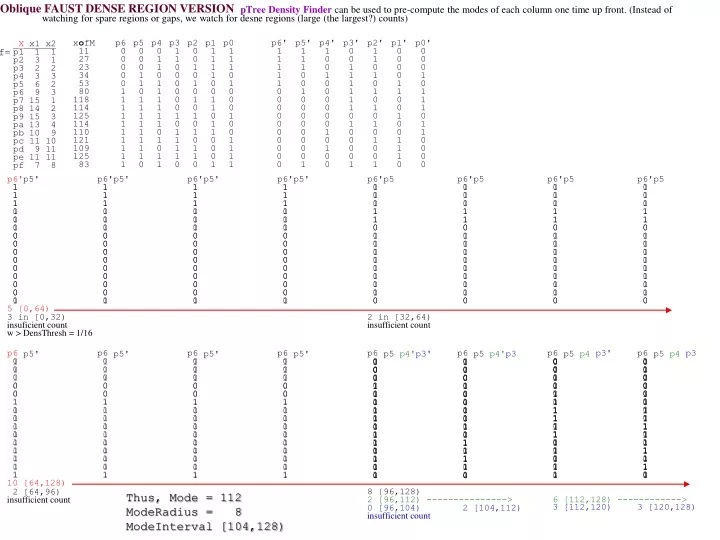
p5' 1 1 1 0 0 1 0 0 0 0 0 0 0 0 1 3 in [0,32) insuficient count w > DensThresh = 1/16 p6' 1 1 1 1 1 0 0 0 0 0 0 0 0 0 0 5 [0,64) p5' 1 1 1 0 0 1 0 0 0 0 0 0 0 0 1 p6' 1 1 1 1 1 0 0 0 0 0 0 0 0 0 0 p6' 1 1 1 1 1 0 0 0 0 0 0 0 0 0 0 p5' 1 1 1 0 0 1 0 0 0 0 0 0 0 0 1 p6' 1 1 1 1 1 0 0 0 0 0 0 0 0 0 0 p5' 1 1 1 0 0 1 0 0 0 0 0 0 0 0 1 p6' 1 1 1 1 1 0 0 0 0 0 0 0 0 0 0 p5 0 0 0 1 1 0 1 1 1 1 1 1 1 1 0 2 in [32,64) insufficient count p5 0 0 0 1 1 0 1 1 1 1 1 1 1 1 0 p6' 1 1 1 1 1 0 0 0 0 0 0 0 0 0 0 p5 0 0 0 1 1 0 1 1 1 1 1 1 1 1 0 p6' 1 1 1 1 1 0 0 0 0 0 0 0 0 0 0 p6' 1 1 1 1 1 0 0 0 0 0 0 0 0 0 0 p5 0 0 0 1 1 0 1 1 1 1 1 1 1 1 0 p3' 0 0 1 1 1 1 1 1 0 1 0 0 0 0 1 3 [112,120) p6 0 0 0 0 0 1 1 1 1 1 1 1 1 1 1 10 [64,128) p6 0 0 0 0 0 1 1 1 1 1 1 1 1 1 1 p6 0 0 0 0 0 1 1 1 1 1 1 1 1 1 1 p6 0 0 0 0 0 1 1 1 1 1 1 1 1 1 1 p6 0 0 0 0 0 1 1 1 1 1 1 1 1 1 1 p6 0 0 0 0 0 1 1 1 1 1 1 1 1 1 1 p6 0 0 0 0 0 1 1 1 1 1 1 1 1 1 1 p3 1 1 0 0 0 0 0 0 1 0 1 1 1 1 0 3 [120,128) p6 0 0 0 0 0 1 1 1 1 1 1 1 1 1 1 p3' 0 0 1 1 1 1 1 1 0 1 0 0 0 0 1 0 [96,104) insufficient count p5' 1 1 1 0 0 1 0 0 0 0 0 0 0 0 1 2 [64,96) insufficient count p5' 1 1 1 0 0 1 0 0 0 0 0 0 0 0 1 p5' 1 1 1 0 0 1 0 0 0 0 0 0 0 0 1 p5' 1 1 1 0 0 1 0 0 0 0 0 0 0 0 1 p5 0 0 0 1 1 0 1 1 1 1 1 1 1 1 0 8 {96,128) p4' 1 0 0 1 0 0 0 0 0 0 1 0 1 0 0 2 [96,112) ---------------> p5 0 0 0 1 1 0 1 1 1 1 1 1 1 1 0 p4' 1 0 0 1 0 0 0 0 0 0 1 0 1 0 0 p3 1 1 0 0 0 0 0 0 1 0 1 1 1 1 0 2 [104,112) p5 0 0 0 1 1 0 1 1 1 1 1 1 1 1 0 p4 0 1 1 0 1 1 1 1 1 1 0 1 0 1 1 6 [112,128) ------------> p4 0 1 1 0 1 1 1 1 1 1 0 1 0 1 1 p5 0 0 0 1 1 0 1 1 1 1 1 1 1 1 0 Oblique FAUST DENSE REGION VERSION pTree Density Finder can be used to pre-compute the modes of each column one time up front. (Instead of watching for spare regions or gaps, we watch for desne regions (large (the largest?) counts) xofM 11 27 23 34 53 80 118 114 125 114 110 121 109 125 83 p6 0 0 0 0 0 1 1 1 1 1 1 1 1 1 1 p5 0 0 0 1 1 0 1 1 1 1 1 1 1 1 0 p4 0 1 1 0 1 1 1 1 1 1 0 1 0 1 1 p3 1 1 0 0 0 0 0 0 1 0 1 1 1 1 0 p2 0 0 1 0 1 0 1 0 1 0 1 0 1 1 0 p1 1 1 1 1 0 0 1 1 0 1 1 0 0 0 1 p0 1 1 1 0 1 0 0 0 1 0 0 1 1 1 1 p6' 1 1 1 1 1 0 0 0 0 0 0 0 0 0 0 p5' 1 1 1 0 0 1 0 0 0 0 0 0 0 0 1 p4' 1 0 0 1 0 0 0 0 0 0 1 0 1 0 0 p3' 0 0 1 1 1 1 1 1 0 1 0 0 0 0 1 p2' 1 1 0 1 0 1 0 1 0 1 0 1 0 0 1 p1' 0 0 0 0 1 1 0 0 1 0 0 1 1 1 0 p0' 0 0 0 1 0 1 1 1 0 1 1 0 0 0 0 X x1 x2 p1 1 1 p2 3 1 p3 2 2 p4 3 3 p5 6 2 p6 9 3 p7 15 1 p8 14 2 p9 15 3 pa 13 4 pb 10 9 pc 11 10 pd 9 11 pe 11 11 pf 7 8 f= p3' 0 0 1 1 1 1 1 1 0 1 0 0 0 0 1 p3 1 1 0 0 0 0 0 0 1 0 1 1 1 1 0 Thus, Mode = 112 ModeRadius = 8 ModeInterval [104,128)
Oblique FAUST DENSE REGION VERSION An Algorithm: 1. Let p = ModeVec = (HighestMode1, HighestMode2, ..., HighestModen) and find each ModRadius. 2. Construct SpTS: SModeVec,r(y)= (y-p) ModeDot (y-p) r2 where y ModeDot p ≡ i=1..n(1/ModRadiusi)(yi-pi)2 3. Increase r until density falls off (first sparse region). Better to look for 1st radial gap (should be one since we;re centering on ModeVec and are constructing fitted ellipsoids around p (fitted via the ModeRadii) 3'. (a better 3): If the density DensityThreshold, peel off SubClusterModeVec,r(y)= (y-p) ModeDot (y-p) 1 as a subcluster and then take the next best p=ModeVec2 and do the same. If ModeVec is the vector of "highest" modes, then ModeVec2 might be a matter of taking the highest CoordinateMode not yet used (say in coordinate, k) and using it instead of the HighestModek in ModeVec. This can, of course, be iterated. So decide on a LowerBoundCoordinateModeThreshold (LBCMT) for declaration of a CoordinateMode. Take all CoordinateModes and sort them descending (remembering which coordinate they came from). For ModeVec1 take the max CoordinateMode in each coordinate. Then iteratively replace the highest CoordinateMode as yet unused to get MideVec2, ModeVec3, etc.. When you run out of CoordinateModes, you can reduce the LBCMT for declaring CoordinateModes and do it all over again. Continue this until we have fully clustered the set (or until the LBCMT falls below some threshold, then declare what's left as the default final subcluster.). Precede all of this with a comprehensive search using linear projections for outliers.
d Oblique FAUST Pipe 1 1. Linear project onto d-line from within a pipe. If no good gaps, start over with new p, d, else if good linear gapped region(s) appear, 2. Look for good radial gaps, use them as in OFP0, If none, for each linear gapped region [xod=a1,xod=a2] (corresp. pts on pd-line are bk=p+akd=pod k=1,2), do: in a narrowed region around p1=avg(b1,b2), incr radius until 1st gap or thinning appears (at r1 Let q1=mean(post-thinning barrel stave ring (radius from r1 to r1 + delta) and let d1=(q1-p1)/|q1-p1| .b2=p+a2d-pod .q1 .p1 .b1=+a1d-pod r1 3. Start over with p1, d1 (more likely to be down the middle of the round cluster and therefore produce barrel gaps (linear and radial)) p Alternatively, one could keep finding points on the sphere (like b1 and b2) until one has n-1 of them (n=dimension of space). Then there is a formula for the center of the circle through those points (at least in low dimensions???). However, even if there is a formula in high dimensions, it would be a nasty one and would take lots of rounds of the above to preduce the n-1 points (~ n/2 rounds). If n=17,000 for instance, that makes it infeasible.
r3 r4 r3 d Oblique FAUST Pipe 2 1. Linear project onto d-line from within a pipe. If no good gaps, reset p, d 2. linear gapped region (mean=m1), increase radius until there appears a region between gaps or thinnings (at r1 and at r2). Let m2=mean(2nd pre-thinning barrel stave). .m2 Let r3=(r2+r1)/2, r4=r2 - r3 Reset d-line thru p'=(r3*m2+r4*m1)/2 r2 .p' 3. Look again for radial gap. if none goto1. 4. If radial gap, restrict to full barrel and look for linear gaps. If none goto 1. 6. If linear gap, declare subcluster, mask off and goto 1. .m1 r1 p
Q&A f=distance dominated functional, avgGap=(fmax-fmin)/|f(X)| may be a good measurement for setting thresholds, e.g., x is an outlier=anomaly if gap around {x} > 3*avgGap? If the minimum barrel radii >> 0, we have chosen a d-line far from the data. It may be advisable to pick p to ba an actual data point. Here are the formulas from the spreadsheet: G=(B12-B$6)*B$9+(C12-C$6)*C$9+(D12-D$6)*D$9+(E12-E$6)*E$9 H=G12-$G$9 L=(x-p)od-min I=(B12-B$6)^2+(C12-C$6)^2+(D12-D$6)^2+(E12-E$6)^2 J=@SQRT(I12-G12^2) B=SQRT[(x-p)o(x-p)-(x-p)od^2] Note we don't round, so we are calculating pTree bitslices by truncating. We don't even need to do that! For fixed piont, here are the bislice formulas: @MOD(@INT(F/2^6),2) @MOD(@INT(F/2^5),2) @MOD(@INT(F/2^4),2) @MOD(@INT(F/2^3),2) @MOD(@INT(F/2^2),2) @MOD(@INT(F/2^1),2) @MOD(@INT(F/2^0),2) Keep going (take bitslices to the right of decimal pt) @MOD(@INT(F/2^-1),2) @MOD(@INT(F/2^-2),2) ... Floating point? Bitslice the mantissa. The exponent shifts the slice name. E.g., .1011 25 .0010 24 .1010 2-1 If d and t are trained over DocumentTerm (DT) Gradient(F)=G=(Gd, Gt). Instead of a LineSearch using F(s)=f +sG, always use 2D-RectangleSearch, F(sd,st)=F(f + sd*Gd + st*Gt). Set F/sd =0 and F/st=0. It may be a better approach to find dense cells (sphere, barrel, cone) then fuse them, because it's difficult to position themaround clusters (due to bumps, protrusion etc.) (Not true for outlier clusters (singleton\doubleton)) An Akg: Start with a line and a small radius barrel around it. Find dense regions between 2 consecutive gaps in this pipe. This should identify portion of a dense cluster. Lots of ways to go from there: a. Use centroid of dense pipe piece as sphere|barrel center. b. Move to a better centroid for that cluster by a gradient asc/desc process c. In a "GA mutation" fashion, jump to a nearby centroid, governed by some fitness function (e.g., count in dense pipe piece). 24 1 0 0 22 1 0 0 21 1 1 0 20 0 0 0 2-1 0 0 0 2-2 0 0 1 2-3 0 0 0 2-4 0 0 1 23 0 0 0 SSPTS = set of all SPTSs (columns of reals); V = n-dim vector space. Code operations on SSPTS (both 1 level or multi-level): 22 2 5/16 SSPTS SSPTS SSPTS (Binary Algebraic Operations): including: +, -, /,RWP =Row_Wise_Product 10110. 10. .01010 {SPTSk}k=1..n SSPTS (Unary ops.Typically SPTSk=Vk) incl: SDv(Square Distance from a fixed vector, vV) Gap analytic tools: L(x)=xod, S(x)=(x-p)o(x-p) and then from those, B(x)=S(x)-L2(x) (If T is the minimum gap threshold, use T2 for S and B ) Oblique FAUST, Barrel (OFLB) Alternate Lpqx, Bpqx to get a cluster dendogram (topdown). Take p=1st_TR pt? d=vomavg Defining Avg Density? AvD = count / k=1..dim(maxk-mink)? This is for choosing good Thresholds. MinGapThres=Tb,AvD≡ b*(1/ AvD)1/dim b=adjustable param If we're given a TrainingSet, TR, with K classes, is avgk=1..Kvomk a better mediod than VoM? Take p=MinCorner, q=MaxCorner of box circumscribing {VoMk}k=1..K better than not circ box of TR? DPv(Dot Product with a fixed vector, vV) ERa= FP's EinRings (n=1, rR) result masks rows s.t. row < a SPTS Rincludes AGa= YC's Aggregates and iceberg queies: count, sum, avg, max, min, median, rank_k, top_k, IceBergQueries. SSPTS SSPTS (Unary Operations) including: SPc=Scalar_Product (Multiply each SPTS row by same constant, c. Use const SPTS? all rows=c, then RWP. More efficient? w/o forming const SPTS? Use c's bit pattern c only? (subset of previous with n = |SSPTS|?) Note, SSPTS includes SPTSs of all cardinalities (= depths = # of rows) It seems best to code on SSPTS rather than on SSPTSn (card(SPTS)=n). Of course, it is very important to know what the rows represent so as to avoid nonsense results, however, why restrict the operations themselves? When SPTS operands are of different depths, the result SPTS's depth = depth of the shallowest operand (operate from the top of each).
M1 H1 L18 M26 H28 C2 M3 L1 M3 H3 C31 L1 M1 H4 C32 H1 M1 H5 C33 H1 H2 M1 M1 M2 M1 H3 C26 L1 L1 M1 d=4 M2 L1 M1 H1 M3 H1 C4 H4 L20 M9 H4 C1 M1 L2 M3 H4C25 L1 L9 M1C21 M1 M3 . H3 L2 M4 H3C23 L1 M1 d=4 . H4 L1 M1 L2 M3 H16C24 H1 M3 M1 L1 M1 L2 M12 H 17 C3 L2 M1 C0 L4 M3 H1C22 L6 L3 M1 C211 H1 L1 M1 ' H3 M2 H2 M1 H1C251 H1 L1 L1 M2 H16 C241 M1 H5 M3 . H1 L1 M1 C231 M1 M1 . H5 M1 . H5 M3 L1 H1 L1 H1 H5 M2 H1 M3 H1 C27 M1 L1 L2 L11 M3 C11 L4 M1 M2 L1 M2 H1 C12 L3 M1 H3 L1 M1 H5 C2411 M2 . H1 L11 M3 L1 M1 L1 L1 H1 M2 if 1st B radius>>0, use p=min_radius_pt OF LB...LBClustering on Concrete(STrength,ConcreteMix,WAter,FineAggregate, AGgregate). Assess STerror L<40M<60H 43 428 228 594 270 43 213 159 904 100 44 428 228 594 365 44 238 187 847 100 44 199 192 826 360 44 140 192 807 180 44 380 228 594 365 45 140 192 807 360 46 375 127 993 7 46 375 127 993 7 46 266 228 670 28 46 374 170 757 7 46 214 182 785 28 47 190 228 670 180 47 214 182 786 56 47 425 151 804 7 47 266 228 670 90 47 531 142 894 7 47 380 154 605 7 48 304 228 670 28 49 304 228 670 90 49 425 154 887 7 49 425 154 887 7 49 266 228 670 180 49 425 154 887 7 60 425 154 887 28 60 375 127 993 56 60 425 154 887 28 60 425 154 887 28 61 374 170 757 28 62 540 162 676 28 62 425 151 804 28 63 374 170 757 56 63 375 127 993 91 64 425 154 887 56 64 425 154 887 56 64 425 154 887 56 65 425 151 804 56 65 374 170 757 91 65 425 154 887 91 65 313 176 612 56 65 425 154 887 91 65 425 154 887 91 66 439 186 708 28 66 319 156 880 56 67 469 138 841 28 67 313 176 612 91 67 425 151 804 91 68 286 145 804 28 68 475 181 782 28 68 319 156 880 91 68 402 147 852 28 68 338 175 756 91 69 469 138 841 56 71 363 165 756 28 71 363 165 756 28 71 363 165 756 28 71 363 165 756 28 71 469 138 841 91 72 475 181 782 56 72 439 186 708 56 73 286 145 804 56 73 439 186 708 91 74 390 146 756 28 74 475 181 782 91 74 402 147 852 56 75 402 147 852 91 75 324 184 660 28 77 363 165 756 56 77 286 145 804 91 77 363 165 756 56 77 363 165 756 56 77 363 165 756 56 79 390 146 756 56 79 363 165 756 91 79 363 165 756 91 79 363 165 756 91 79 363 165 756 91 80 324 184 660 56 83 390 146 756 91 (x-p)od/4 gp3 C11 15 1 2 17 1 3 20 1 1 21 1 1 22 3 1 23 1 1 24 2 1 25 1 4 29 3 (x-p)od/4 gp3 C21 35 1 1 36 1 1 37 2 1 38 1 1 39 1 3 42 3 1 43 1 (x-p)od/4 Ct Gp3 C p 140 192 807 3 T=MGW=12 d=x-n=.58 .15 .58 .53 CONCRETE ST CM WA FA AG 8 140 192 807 3 8 168 122 780 3 9 190 162 803 3 10 310 192 851 3 20 230 195 759 14 20 238 187 847 3 21 212 180 779 14 21 191 162 804 14 22 166 176 780 28 22 234 198 852 14 22 230 195 758 14 23 234 198 852 28 23 190 162 803 14 23 363 165 756 7 24 168 122 780 28 24 338 175 756 3 24 286 145 804 3 24 222 189 870 14 24 230 195 759 28 25 319 156 880 3 25 222 189 870 28 25 230 195 758 28 25 195 166 906 14 25 212 180 779 28 25 166 176 780 14 25 250 187 861 14 26 191 162 804 28 26 195 166 906 28 26 238 228 594 7 26 238 187 847 14 26 213 159 904 14 28 190 162 803 28 28 389 158 926 3 28 234 198 852 56 28 199 192 826 28 28 140 192 807 28 28 324 184 660 3 29 380 154 605 3 29 375 127 993 3 29 313 176 612 3 29 250 187 861 28 29 166 176 780 56 29 222 189 870 56 40 214 182 786 28 40 190 162 803 100 40 469 138 841 3 40 238 187 847 56 40 333 228 594 270 40 212 180 779 100 41 333 228 594 365 41 390 146 756 3 41 222 189 870 100 41 191 162 804 100 41 531 142 894 3 41 190 228 670 28 41 380 228 594 90 41 380 228 594 270 41 380 228 594 180 41 230 195 758 100 41 402 147 852 3 42 475 228 594 270 42 190 228 670 90 42 428 228 594 90 42 475 228 594 90 42 475 228 594 365 42 199 192 826 180 42 428 228 594 180 42 250 187 861 100 43 213 159 904 56 43 475 228 594 180 43 313 176 612 7 Br/4 gp3 C211 0 1 4 4 1 3 7 1 3 10 1 Br/4 gp3 C0 19 2 46 65 1 0 1 7 7 1 4 11 2 1 12 1 3 15 4 2 17 1 1 18 3 1 19 2 1 20 2 1 21 1 1 22 6 1 23 3 1 24 4 1 25 2 1 26 1 1 27 2 2 29 2 3 32 2 1 33 3 1 34 2 1 35 1 1 36 2 1 37 3 1 38 3 1 39 5 1 40 2 1 41 2 1 42 8 1 43 1 1 44 2 1 45 3 1 46 6 1 47 2 1 48 2 1 49 3 1 50 2 1 51 8 2 53 1 1 54 1 1 55 1 1 56 3 1 57 1 1 58 3 3 61 2 1 62 3 1 63 2 2 65 1 1 66 2 1 67 5 1 68 1 1 69 1 1 70 5 1 71 1 2 73 1 1 74 6 1 75 1 3 78 4 3 81 1 1 82 1 1 83 2 3 86 1 Br/4 gp3 C1 0 1 5... 7 1 3... 21 1 3 24 4 19 43 1 4 47 1 4... 53 1 3... 59 1 7... 68 1 10... 79 1 (x-p)od/4 gp3 C23 30 3 4 34 1 3 37 1 4 41 1 4 45 1 5 50 1 1 51 1 (x-p)od/4 gp3 C12 20 1 3 23 1 4 27 2 Br/4 gp3 C231 0 1 35 35 1 (x-p)od/4 gp3 C22 38 1 1 39 1 1 40 1 5 45 1 3 48 1 3 51 1 1 52 1 5 57 1 Br/4 gp3 C241 0 1 2 ... 4 4 5 9 1 1 10 4 6 16 1 1 17 4 3 20 1 41 61 1 (x-p)od/4 g3 C411 13 1 9 21 5 Br/4 gp3 C2 0 1 3 3 1 1 ... 8 1 5 13 1 3 16 2 1 18 3 3 21 1 1 ... 26 2 3 29 1 7 36 1 2 ... 43 2 3 46 2 1 ... 48 2 3 51 1 9 60 1 2 62 3 13 75 1 7 82 1 1 83 1 4 87 1 1 ... 91 1 3 94 2 Br/4 gp3 C251 0 1 25 25 1 (x-p)od/4 gp3 C24 36 1 3 39 1 2 ... 53 1 5 58 1 (x-p)od/4 gp3 C25 38 1 4 42 1 3 45 1 4 49 1 5 54 1 1 55 1 3 58 1 (x-p)od/4 gp3 C26 46 1 3 49 1 2 51 1 5 56 1 (x-p)od/4 gp3 C27 46 1 3 49 1 2 51 1 5 56 1 (x-p)od/4 gp3 C33 0 1 30 30 4 2 32 1 Br/4 ct gp3 C3 0 1 13 13 3 1 14 3 3 17 5 2 19 1 4 23 1 6 29 2 1 30 2 2 32 1 2 34 1 4 38 1 4 42 1 2 44 1 3 47 1 57 104 1 4 108 1 2 110 1 3 113 1 11 124 3 (x-p)od/4 gp3 C31 67 3 3 70 3 (x-p)od/4 gp3 C32 0 2 32 32 3 2 34 1 c(Clust dendogram w/o purity) c0 c1 c2 c3 c4 c31 c32 c33 c11 c12 c21 c22 c23 c24 c25 c26 c27 c251 c211 c231 c241 c2411 Br/4 ct gp3 C4 40 1 33 73 1 1 74 1 42 116 1
Oblique FAUST (OF)Clustering:Linear (default) OFL,Spherical OFS, Barrel OFB, Conical OFC) a2 Bpdx a1 x r d p d No gaps show on the red, blue or green projection lines Note: Bpd(x) = Sp(x) - L2pd(x) Cp,d(x)=(x-p)od / (x-p)o(x-p) Oblique FAUST Cone (OFC)(Enclose clusters with cone gaps) GapLower GapUpper Note: C2pd(x) = L2pd(x) /Sp(x) p p gapBarrel Assume a real number table, T, converted to a PTreeSet. Each method uses a real valued functional from X to R and all methods are completely data parallel (data can be distributed over a cluster, processed in parallel (dot product), then the partial results sent home to be added. Lp,d:XR: Lp,d(x)=(x-p)od Oblique FAUST Linear (OFL) clustering (Enclose clusters between (n-1)-dimensional hyperplanar gaps) Find a1<a2 such that =GapLower={x | a1<Lpd(x)<a1+T}and =GapUpper={x | a2<Lpd(x)<a2+T}and C={x|a1+T<Lpd(x)<a2} Bp,d(x)=(x-p)o(x-p)-((x-p)od)2Oblique FAUST Barrel (OFB)(Enclose clusters with barrel gaps) Search for GapLower>T, GapUpper>T and GapBarrel>T2 (BR≡Barrel_Radius) Sp(x)=(x-p)o(x-p) Oblique FAUST Spherical (OFS)(Enclose clusters with spherical gaps) Search Sp for spherical gap, {x | r2 Sp(x) < (r+T)2}= so that the interior of the r-sphere about p encloses a sub-cluster.
4.5<F<7.5 R Ct gp 0 3 10 10 3 4 14 5 6 20 4 2 22 7 6 28 1 2 30 9 2 32 6 10 42 2 5 47 1 13 60 2 Oblique FAUST Pipe 0 Clustering on SEEDS( Thinning1 45 2 48 42 72 Thinning2 5 36 2 0 12 0 pipe 4 34 0 1 2 2 0 0 12 40 2 2 5 0 3 0 0 31 d p=minq=max ClsAreaLnkeAcoeLnk) 1 15 6 2 5 1 15 6 1 5 ... 3 12 5 6 5 F<4.5 R Ct gp 0 5 10 10 9 4 14 13 3 17 3 3 4.5<F<7.5 R Ct gp 17 3 5 22 1 2 ... MinRad too high! reset p xod Ct gp 0 3 1 1 17 1 2 39 1 3 26 1 4 10 1 5 10 1 6 17 1 7 16 1 8 6 1 9 3 1 10 3 xod Ct gp in pipe 2 8 1 3 14 1 4 5 1 region! Look for radial gaps xod Ct gp in pipe 2 8 1 3 14 1 4 5 1 region! Look for radial gaps R Ct gp 0 5 10 10 9 4 14 13 3 17 3 3 20 1 2 22 8 2 24 5 4 28 1 2 30 4 2 32 2 1 33 1 4 37 11 5 42 2 2 44 10 2 46 8 5 51 4 3 54 1 3 57 4 2 59 1 6 65 1 8 73 1 The alg only specifies looking at the first region, but it is interesting that other clusters are revealed Next, Lin gap anal in r=26 barrel. xod Ct gp 1 5 1 2 11 1 3 20 1 4 8 1 5 7 p Notes: 1. OFP0 may not work well if the pipe runs through the edge of a round cluster. The philosophy is the probabilistically, pipes are more likely to run through the center region of a round cluster since there is more of it. Next we try ways of adjusting p so that the pipe is more in the center of the subcluster. 2. I also tried Spherical when it appeared from the pipe analysis that we were at the center of a cluster. So far this didn't work out. 0. Always start with a pd-line linear gap analysis, then: 1. Find gapped regions in pipe: Project inside of pd-pipe (small radius). full linear gapped region, analyze for an Initial Radial Gap (IRG). 2. If IRG, increase linear region width until cap gaps appear.. 3. Mask off that cluster 4. GOTO 1, using revise p,d at this point or if either 2, 3 have no gaps
Oblique FAUST Pipe 01Clustering on SEEDS 34 23 1 p=nnnn q=xxxx R Ct gp 0 8 1 1 50 1 2 38 1 3 20 1 4 18 1 5 7 1 6 8 1 7 1 r0=1.5 pipe L Ct gp 2 2 1 3 7 1 4 5 No thinnings so it's just one dense region In middle of dense portion, [=3], find radial falloff, r1 R Ct gp 0 5 10 10 2 4 14 7 3 17 3 5 22 3 6 28 1 9 37 1 14 51 1 8 59 1 6 65 1 8 73 1. Linearly project in a pdr0-pipe. 2. For every very dense region (take just the most dense middle portion? Find first radial density falloff at r1. If none GOTO 5. 3. Linearly project pdr1 barrel to determine the linear extent of that dense region. If it fails to show up. GOTO 5. 4. Mask off that cluster 5. Revise p and d and GOTO 1.
US≡Universe of Scalar pTreeSetsA ScalarpTreeSet is the complete set of pTrees for a column of real numbers (Complete: a pTree bit pos, - to ToC entry for a SpTSs in a RBaDB Real BitarrayDataBase predicate? level=? depth=? Min=? Rank¼ Median=Rank½? Rank¾> Max=? Sum=? bit posptr|purity1count (n+1,) pure0 0 n pointern146374 n-1 pointern-19284 ... n' pure1 depth ... n" pure0 0 ... -m pointer-m48293847 (-,-m-1) pure0 Notes: 0. pointerk =pointer to a bit vector. 1.1st and last rows can be implied? 2. Other cols? (e.g., Identical Twins) 3. Need separate ToC for PTreeSets (as sequences of same-depth SpTSs for tables of real numbers). 4. It's OK to black box SpTSs as real columns since then complex columns can be defined at a higher ToC level via pointers to their real and complex parts. 5. To mult by 2k shift bit pos defs only. So a cleaner ToC might be: How do we define (black box) ScalarpTreeSets (SpTSs) in a ToC or VDB Catalog? |SpTSresult| ≡ depth = min{|SpTS1|,..., |SpTSm|} n-ary operations: US...USUS add (row-wise) SpTS1+...+ SpTSm SpTSresult SpTSresult,k=SpTS1,k+..+SpTSm,k -, /,* are similarly defined row_wise operations. =, >, <, , are binary ops producing mask pTree (i.e., bitwidth(SpTSresult)=1 SPc=Scalar Product (multiplying every row of an SpTS by a constant, c). One can use * above or possibly, use c's bit pattern to avoid constructing a constant SpTS) DPv:=Dot Product with a fixed real vector, vV Again, use v's bit pattern? SDv=Square Distance from fixed real vector, vV Again use v's bit pattern only? ERa= EinRings = pTree mask of rows < a apply < above? Better, use a's bit pattern only? AGa= YC's Aggregates, count, sum, avg, max, min, median, rank_k, top_k, IceBergQueries (Here, the result is a number, but a number is a depth=1, width=1 SpTS.) ToC for SpTSs in a RBaDB predicate? .. Sum? Highest_NonPure0_Bit_Position=n PointerArray=( ptr(n),...,ptr(-m) ) CountArray=( cnt(n),...,cnt(-m) ) I.e., use offsets instead of keywords to implement the pTree pointer table. Some red info is redundant. How much pre-computed (redundant?) info should be placed in the ToC? Rules of thumb: Pre-compute everything that might be useful and certainly pre-compute all info that might require Horizontal Processing of Vertical pTrees. I believe Min, Med, Max, Sum can be derived from ToC info (the counts) without accessing actual pTrees and thus, should be store in the ToC only if doing so save significant processing time.
Oblique FAUST with a comprehensive initial linear step (done in parallel?) n1y1+ x2y2+ n3y3+ x4y4+ x1y1+ n2y2+ x3y3+ n4y4 or p and q from side-mid-pt to a opposite corner (n2n-1 = 32) aaan - anaa - xxxx xxxn xxnx xxnn nxxx nxxn nxnx nxnn naaa - xxxx xxxn xxnx xxnn xnxx xnxn xnnx xnnn xxxx xxnx xnxx xnnx nxxx nxnx nnxx nnnx aana - xxxx xxxn xnxx xnxn nxxx nxxn nnxx nnxn I have not used column numbers. e.g., n=minimum means n is a number and it is the minimum of a column of numbers (indicated here by the position in which it appears, not by subscript (offset, not keyword identification of the column)). Each of n,x,a,m are width=4 vectors or 4-tuples of numbers, so they are: (n1, n2, n3, n4) For table,Y=(Y1.Y2.Y3.Y4), let n=minYk, x=maxYk a=avgYk m=medianYk k=1|2|3|4 yY, Lpq(y)=(y-p)o(q-p/|p-q|), p,q any of p and q form diagonals: nnnn - xxxx nnnx - xxxn nnxn - xxnx nnxx - xxnn nxnn - xnxx nxnx - xnxn nxxn - xnnx nxxx - xnnn xnnn - nxxx xnnx - nxxn xnxn - nxnx xnxx - nxnn xxnn - nnxx xxnx - nnxn xxxn - nnnx xxxx - nnnn (x1, x2, x3, x4) (a1, a2, a3, a4) (m1, m2, m3, m4) As on slide 1, these are precomputed and stored as ToC info 0 1 2 3 4 5 6 7 8 9 a b c d e f yY = PTreeSet for a table of reals, for any of the 44 (p,q), then in a first dot product with (q-p) step do all 44 dot products and gap analyses! Lot of work? Yes, but there is computational parallelism (Note there is no need to insist on unit vectors - we can dot with q-p and then realize that the gaps will be |q-p| wider than they would have been, had we used dpq instead (affects choice of threshold only)). So if p=(n1, x2, n3, x4) then q=(x1, n2, x3, n4), and then precomputed fixed vectorss (y-p)o(q-p)=yoq-yop-poq+pop= (y1y2y3y4)o(n1,x2,n3,x4)- (y1y2y3y4)o(x1,n2,x3,n4)-poq+pop 8 thru f are the same diagonals as 7 thru 0, so we only need 2n-1 =8 0 thru 7 So if, given Y pre-compute all these scalar-times-SpS binary multiplications of Yk with the 16 pre-computed numbers, nk, xk, ak and mk, then any of these dot product SpSs is a 8-sum of those we precomputed and is thus not much work (4*45=180 8-sums). It may be possible to engineer 8-summing process to cut time even further? Or to engineer an efficient way to do 8 scalar multiplications and the 8-summings in one efficient operation. Of course, it won't always be 8. For the Netflix Movie PTreeSet, there are 17,000 columns, not 4; and for the User PTreeSet there are 500,000. or p and q midlines combo(n,n-1) of them =n!/(n-(n-1))!(n-1)!=n=4 aaan - aaax aana - aaxa anaa - axaa naaa - xaaa If finding outliers (anomalies), since most anomalies occur at the outside boundaries of a set, this simple method might find all of them without further processing. The other aspect of OF that needs attention is making this local in the sense that clusters are revealed by local application of linear gap analysis even though for the entire space, no gaps appear. This is the reason to introduce barrel gaps if the initial linear gap analysis fails. By substituting m for a (median for avg) we could get 32 more, but they seem likely to be essentially the same lines as given by a? Possibility: Always use m instead of a as a center? 32 mdpt-corner are more and more distinct from the diagonals as the dimension increases. There are (n+1)(2n-1+1) (p,q) pairs to consider.
Oblique FAUST a comprehensive initial linear step using a central point, p ox tx or q: o=Rank¼, t=Rank¾ pt (n2n-1) tttx ttox totx toox ottx otox ootx ooox ttxt ttxo toxt toxo otxt otxo ooxt ooxo txtt txto txot txoo oxtt oxto oxot oxoo xttt xtto xtot xtoo xott xoto xoot xooo mx xx xn For Y=(Y1.Y2.Y3.Y4), n=minYk, x=maxYk m=medYk o=rank¼Yk t=rank¾Ykk=1|2|3|4 yY, Lpq(y)=yo(q-p)/|q-p|, p=central pt= the1st pt in the 1st ring around p in SVoM(Y) q is any of (2n-1 of them) xxxx xxxn xxnx xxnn xnxx xnxn xnnx xnnn xt p xm xo What we are attempting to do here is get a full coverage of ~evenly spaced projection lines (pq-lines or d-lines). We are doing so by attempting to evenly space q on [half of] the sides. That seems easier than evenly spacing points on [half of] the sphere (using angles) If dim=N is high, there may be unevenness to this method? However, using rank(k/N), k=1..N-1 instead of length increments by =(max-min)/N should ameliorate that? We can calculate the ranks using our logn pTree rank procedures. Furthermore, once we move to barrel gapping to limit the radial reach (and therefore materialize gaps for large dataset that would not appear with just linear analysis), using an actual point in the set as p has definite advantages (always centers the barrel on actual points in the space so we get a r=0 radius every time). or q: m=median pt = Rank½ (n of them) mmmx mmxm mxmm xmmm Oblique FAUST 2nd Barrel step (paralleling?) 1. L(q-p)/|q-p|(y)=(y-p)o(q-p)/|q-p| find outliers and linearly gapped clusters. (1/|q-p|=a) 2. Then look for barrel gaps around all dense regions (between thinnings) using Sp(y)=(y-p)o(y-p)= yoy -2yop +pop and B(q-p)/|q-p|(y)=Sp(y)-L(q-p)/|q-p|(y)2 = yoy -2yop + pop - (yop-yoq-poq+pop)2/a2 Every dot product in the above is a linear combination of SpSs of the form, b*Yk for some b{n.x,a,0,m,t}. Thus, if we precompute those SpSs we can put together L and B projections efficiently.
f=p1 and xofM-GT=23. First round of finding Lp gaps p5' 1 1 1 0 0 1 0 0 0 0 0 0 0 0 1 p4' 1 0 0 1 0 0 0 0 0 0 1 0 1 0 0 p4' 1 0 0 1 0 0 0 0 0 0 1 0 1 0 0 p4' 1 0 0 1 0 0 0 0 0 0 1 0 1 0 0 p5' 1 1 1 0 0 1 0 0 0 0 0 0 0 0 1 p5' 1 1 1 0 0 1 0 0 0 0 0 0 0 0 1 p6' 1 1 1 1 1 0 0 0 0 0 0 0 0 0 0 p5' 1 1 1 0 0 1 0 0 0 0 0 0 0 0 1 p6' 1 1 1 1 1 0 0 0 0 0 0 0 0 0 0 p6' 1 1 1 1 1 0 0 0 0 0 0 0 0 0 0 p4' 1 0 0 1 0 0 0 0 0 0 1 0 1 0 0 p6' 1 1 1 1 1 0 0 0 0 0 0 0 0 0 0 p6' 1 1 1 1 1 0 0 0 0 0 0 0 0 0 0 p6' 1 1 1 1 1 0 0 0 0 0 0 0 0 0 0 p5' 1 1 1 0 0 1 0 0 0 0 0 0 0 0 1 p6' 1 1 1 1 1 0 0 0 0 0 0 0 0 0 0 p6' 1 1 1 1 1 0 0 0 0 0 0 0 0 0 0 p5' 1 1 1 0 0 1 0 0 0 0 0 0 0 0 1 p4' 1 0 0 1 0 0 0 0 0 0 1 0 1 0 0 p4' 1 0 0 1 0 0 0 0 0 0 1 0 1 0 0 p5' 1 1 1 0 0 1 0 0 0 0 0 0 0 0 1 p4' 1 0 0 1 0 0 0 0 0 0 1 0 1 0 0 p4' 1 0 0 1 0 0 0 0 0 0 1 0 1 0 0 p5' 1 1 1 0 0 1 0 0 0 0 0 0 0 0 1 p3' 0 0 1 1 1 1 1 1 0 1 0 0 0 0 1 p4 0 1 1 0 1 1 1 1 1 1 0 1 0 1 1 p4 0 1 1 0 1 1 1 1 1 1 0 1 0 1 1 p4 0 1 1 0 1 1 1 1 1 1 0 1 0 1 1 p4 0 1 1 0 1 1 1 1 1 1 0 1 0 1 1 p4 0 1 1 0 1 1 1 1 1 1 0 1 0 1 1 p4 0 1 1 0 1 1 1 1 1 1 0 1 0 1 1 p4 0 1 1 0 1 1 1 1 1 1 0 1 0 1 1 p4 0 1 1 0 1 1 1 1 1 1 0 1 0 1 1 p5 0 0 0 1 1 0 1 1 1 1 1 1 1 1 0 p5 0 0 0 1 1 0 1 1 1 1 1 1 1 1 0 p5 0 0 0 1 1 0 1 1 1 1 1 1 1 1 0 p5 0 0 0 1 1 0 1 1 1 1 1 1 1 1 0 p5 0 0 0 1 1 0 1 1 1 1 1 1 1 1 0 p5 0 0 0 1 1 0 1 1 1 1 1 1 1 1 0 p5 0 0 0 1 1 0 1 1 1 1 1 1 1 1 0 p5 0 0 0 1 1 0 1 1 1 1 1 1 1 1 0 p3' 0 0 1 1 1 1 1 1 0 1 0 0 0 0 1 p3 1 1 0 0 0 0 0 0 1 0 1 1 1 1 0 p3 1 1 0 0 0 0 0 0 1 0 1 1 1 1 0 p3' 0 0 1 1 1 1 1 1 0 1 0 0 0 0 1 p3' 0 0 1 1 1 1 1 1 0 1 0 0 0 0 1 p3 1 1 0 0 0 0 0 0 1 0 1 1 1 1 0 p3 1 1 0 0 0 0 0 0 1 0 1 1 1 1 0 p3' 0 0 1 1 1 1 1 1 0 1 0 0 0 0 1 p3' 0 0 1 1 1 1 1 1 0 1 0 0 0 0 1 p6 0 0 0 0 0 1 1 1 1 1 1 1 1 1 1 p6 0 0 0 0 0 1 1 1 1 1 1 1 1 1 1 p6 0 0 0 0 0 1 1 1 1 1 1 1 1 1 1 p6 0 0 0 0 0 1 1 1 1 1 1 1 1 1 1 p6 0 0 0 0 0 1 1 1 1 1 1 1 1 1 1 p6 0 0 0 0 0 1 1 1 1 1 1 1 1 1 1 p6 0 0 0 0 0 1 1 1 1 1 1 1 1 1 1 p6 0 0 0 0 0 1 1 1 1 1 1 1 1 1 1 p3 1 1 0 0 0 0 0 0 1 0 1 1 1 1 0 p3 1 1 0 0 0 0 0 0 1 0 1 1 1 1 0 p3' 0 0 1 1 1 1 1 1 0 1 0 0 0 0 1 p3' 0 0 1 1 1 1 1 1 0 1 0 0 0 0 1 p3 1 1 0 0 0 0 0 0 1 0 1 1 1 1 0 p3 1 1 0 0 0 0 0 0 1 0 1 1 1 1 0 pTree Gap Finder can also be used to find the mode(s) of the distribution of F values! Instead of watching for spareness (and ultimately a zero count) we watch for large (the largest?) counts xofM 11 27 23 34 53 80 118 114 125 114 110 121 109 125 83 p6 0 0 0 0 0 1 1 1 1 1 1 1 1 1 1 p5 0 0 0 1 1 0 1 1 1 1 1 1 1 1 0 p4 0 1 1 0 1 1 1 1 1 1 0 1 0 1 1 p3 1 1 0 0 0 0 0 0 1 0 1 1 1 1 0 p2 0 0 1 0 1 0 1 0 1 0 1 0 1 1 0 p1 1 1 1 1 0 0 1 1 0 1 1 0 0 0 1 p0 1 1 1 0 1 0 0 0 1 0 0 1 1 1 1 p6' 1 1 1 1 1 0 0 0 0 0 0 0 0 0 0 p5' 1 1 1 0 0 1 0 0 0 0 0 0 0 0 1 p4' 1 0 0 1 0 0 0 0 0 0 1 0 1 0 0 p3' 0 0 1 1 1 1 1 1 0 1 0 0 0 0 1 p2' 1 1 0 1 0 1 0 1 0 1 0 1 0 0 1 p1' 0 0 0 0 1 1 0 0 1 0 0 1 1 1 0 p0' 0 0 0 1 0 1 1 1 0 1 1 0 0 0 0 X x1 x2 p1 1 1 p2 3 1 p3 2 2 p4 3 3 p5 6 2 p6 9 3 p7 15 1 p8 14 2 p9 15 3 pa 13 4 pb 10 9 pc 11 10 pd 9 11 pe 11 11 pf 7 8 f= OR between gap 2 and 3 for cluster C2={p5} width=23 =8 gap: [010 1000, 010 1111] =[40,48) width=23=8 gap: [000 0000, 000 0111]=[0,8) width=23 =8 gap: [011 1000, 011 1111] =[56,64) width = 24 =16 gap: [100 0000, 100 1111]= [64,80) width= 24 =16 gap: [101 1000, 110 0111]=[88,104) OR between gap 1 & 2 for cluster C1={p1,p3,p2,p4} between 3,4 cluster C3={p6,pf} Or for cluster C4={p7,p8,p9,pa,pb,pc,pd,pe} No zero counts yet (=gaps)
Oblique FAUST SPARCE REGION VERSION (initial linear step): Ways to handle negatives generated in dot product projection step. 1. Only pair p with d if (y-p)od 0 2. Use sign mask to separate into 2 parts (positive part, negative part) then analyze whether there's a gap at 0. 3. After computing SpTS which represents the dot product result and is expressed in 2's complement, before converting to regular decimal bitslice pTrees, compute the minimum and subtract it from the result. Then convert to a decimal bitslice PTreeSet. 1. Mini1..ik≡ vector with minYh at pos h for h=1i ..ik and maxYh elsewhere (MinVec=Min1..n MaxVec=Min-) For d=ek, k=1..n, use p=MinVec For d=Diagonali1..1k≡(q-p)/|q-p|, where p=Mini1..ik and q=Mincomp{i1..ik} , use p. In the Barrel method it is paramount to locate the barrel carefully. Find mode(s) of every column (use pTree Gap Finder, but watch for denseness, not sparseness (next slide)). For the column, k, with the maximum density at the mode, let d=ek Let p=VecMod≡(modeY1,...,modeYn) Let's take our pulse wrt the first linear FAUST step (done prior to any barrel-based reach limitation masking) 1. Exhaustive search for a good unit vector, d (producing good linear gaps): Sequence thru d's (pairing each with a starting pt, p, s.t. (Y-p)od 0 or separately in the negative range, around 0, in the positive range. Take d{e1..en}, p=MinVec. Take d{DiagCC=1..n C{1..n}. DiagCc = unit diagonal from the corner, p, w pk=MinYk kc else pk=MaxYk, to the corner, q, qk=MaxYk kc, else qk=MinYk (no negatives).. When MidPts of sides and hypersides are used for p and/or q, care must be taken in picking p since negatives can appear. 2. Selective choices of d: ModeVec seems very valuable (along with MedVec and Mean.)