Download
1 / 27
270 likes | 383 Views
MODEL.LA Modeling Laboratory This guided introduction (produced from screen captures of the actual program) will provide an overview of the modeling capabilities of MODEL.LA . To advance through this tour, please press the right arrow key ( ) on your keyboard, or click the left mouse button.

E N D
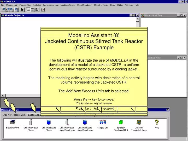
MODEL.LA • Modeling Laboratory • This guided introduction (produced from screen captures of the actual program) will provide an overview of the modeling capabilities of MODEL.LA. • To advance through this tour, please press the right arrow key () on your keyboard, or click the left mouse button. • To replay a portion of this tour, please press the left arrow key () on your keyboard until the desired location is reached. • To quit the tour at any time, press the escape key (Esc) on your keyboard. • Press the key to continue. • The MODEL.LA Modeling Methodology • MODEL.LA contains no predefined models. Rather it leads students through a structured sequence of modeling • decisions--decisions the student makes based on the context of some engineering problem. • From these decisions, MODEL.LA will automatically derive the necessary modeling equations and guide the student through their numerical solution. • Thus, the educational focus shifts from textbook equation selection and solution, to the richer task of model formulation and analysis of process behavior. • Press the key to continue. • Press the key to review. • Modeling Assistant • A rich body of chemical engineering science exists and is currently taught to students in the context of abstract idealized examples. Modeling unifies these scientific principles in their application to real engineering problems. • Unfortunately, students are never taught a modeling methodology. Rather they are forced to infer modeling techniques from exposure to example after example. • The Modeling Assistant of MODEL.LA provides the starting point which guides the student in applying classic classroom concepts in a structured process of model development. • Press the key to continue. • Press the key to review. Modeling Assistant (8) When the physico-chemical phenomena-based description of the model is complete, MODEL.LA automatically derives the corresponding mathematical equations based on chemical engineering first principles. Solution of these equations allows the student to analyze the resulting behavior of the process, appreciate the relationship between phenomena and behavior, and gain immediate feedback on the applicability of the model. At any point the student is free to revisit the assumptions made, make changes, provide additional details, etc. Press the key to continue. Press the key to review. • Modeling Assistant (2) • Models are much more than just equations. They are a concise representation of a real process. The most important step in model development is not the selection of equations from a textbook, but rather the identification and characterization of the relevant physical and chemical phenomena assumed to occur in the process. • Model development begins with identification of control volumes of interest. • Press the key to continue. • Press the key to review. Jacketed Continuous Stirred Tank Reactor (CSTR) Example The following will illustrate the use of MODEL.LA in the development of a model of a Jacketed CSTR--a uniform continuous flow reactor surrounded by a cooling jacket. The modeling activity begins with declaration of a control volume representing the Jacketed CSTR. The Add New Process Units tab is selected. Press the key to continue. Press the key to review. • Modeling Assistant (3) • It continues with perception of how these control volumes interact through transport of material, energy, and chemical species. • Press the key to continue. • Press the key to review. Modeling Assistant (6) The mechanisms which drive the transport of material, energy, and chemical species are characterized. Press the key to continue. Press the key to review. Modeling Assistant (4) The relevant chemical species and reactions must be identified. Press the key to continue. Press the key to review. Modeling Assistant (7) External control actions may be applied. Press the key to continue. Press the key to review. Modeling Assistant (5) The control volumes are further characterized and refined. Press the key to continue. Press the key to review.
Naming of Jacketed_Cstr and the default name Unit0 is changed to Jacketed_CSTR. Press the key to continue. Press the key to review. Hierarchical Tree Flowsheet Context-Sensitive Right-Click Menus A right button mouse click on the modeled unit icon activates a context- sensitive menu listing all options available for that particular modeled-unit. Press the key to continue. Press the key to review. Naming of Jacketed_Cstr The Rename option is selected. Press the key to continue. Press the key to review. Resize Icon The icon for the Jacketed_CSTR is resized. Press the key to continue. Press the key to review. Properties View Declaration of CSTR Control Volume The Blackbox Unit Icon is selected (meaning no internal detail will initially be present in the unit). Press the key to continue. Press the key to review. Declaration of CSTR Control Volume The modeled unit is added to the flowsheet. The Hierarchical Tree pane lists all modeled units in the model. The Properties View lists all assumptions made regarding the currently selected modeled unit Press the key to continue. Press the key to review.
Load Icon and the option to load a new icon is selected. Press the key to continue. Press the key to review. Load Icon Graphical icons do not introduce any new assumptions to the model, but allow the modeler to provide visual clues to the purpose of a model. Press the key to continue. Press the key to review.
Declaration of Interactions with Surroundings and adding it to the flowsheet. Press the key to continue. Press the key to review. Declaration of Interactions with Surroundings A feed stream of reactants enters the Jacketed_Cstr from the surroundings. This is declared by selecting the Add New Fluxes tab of the Modeling Assistant, selecting the Convective Flux Icon... Press the key to continue. Press the key to review. Naming of Feed Stream The feed stream is renamed reactants_input. This is accomplished by selecting the Edit Fluxes tab of the Modeling Assistant, selecting the Rename Flux Icon... Press the key to continue. Press the key to review. Declaration of Interactions with Surroundings The product stream, products_output, transports material from the reactor to its surroundings. It is added and named is a similar manner. Press the key to continue. Press the key to review. Declaration of Interactions with Surroundings Flows of coolant from (coolant_inlet) and to (coolant_outlet) the surroundings are also declared. Press the key to continue. Press the key to review. Naming of Feed Stream and entering the desired name. Press the key to continue. Press the key to review. Press the key to continue. Press the key to review.
Refinement of Jacketed_Cstr At the current level of detail, the student realizes that there is no way to state that the reaction mixture and cooling jacket fluid are in separate vessels within the Jacketed_Cstr. Therefore, the structure of the Jacketed_Cstr must be refined by selecting the Edit Process Units tab and selecting the Specify Internal Subunits option. Press the key to continue. Press the key to review. Review of Assumptions The Properties View is automatically updated after each modeling declaration. Press the key to continue. Press the key to review.
Refinement of Jacketed_Cstr The Hierarchical Tree reflects the refinement of the Jacketed_Cstr into a Vessel and Jacket. Press the key to continue. Press the key to review. Load Icon A graphic icon representing the Vessel is selected. Press the key to continue. Press the key to review. Naming of Vessel The subunit is renamed Vessel. Press the key to continue. Press the key to review. Refinement of Jacketed_Cstr This activates the refinement flowsheet for the Jacketed_Cstr. The abstract boundary of the Jacketed_Cstr is represented by the dashed line. Fluxes to/from the unit initially appear terminating at this boundary. New units added within this boundary are subunits of the abstract unit. Press the key to continue. Press the key to review. Refinement of Jacketed_Cstr Refined subunits are again added using the AddNew Process Units of the Modeling Assistant. In this case, the first subunit is assumed to contain a single liquid phase. Press the key to continue. Press the key to review. Refinement of Jacketed_Cstr The second subunit is added to the Jacketed_Cstr... Press the key to continue. Press the key to review. Refinement of Jacketed_Cstr The subunit is added to the Jacketed_Cstr. Press the key to continue. Press the key to review. Jacket the subunit is renamed Jacket, and a new icon loaded. Press the key to continue. Press the key to review.
Flux Mechanism A Surface Convection flux mechanism is selected, where the heat exchanged is proportional to the temperature difference between the Vessel and the Jacket. Press the key to continue. Press the key to review. Declaration of Internal Interaction and dragging on the refinement flowsheet from the Vessel to the Jacket. Press the key to continue. Press the key to review. Flux Mechanism The amount of heat exchanged is not known in advance. It is determined by a temperature differential between the Vessel and the Jacket. Flux mechanism are declared using the Edit Flux Properties option on the Edit Fluxes tab of the Modeling Assistant Press the key to continue. Press the key to review. Naming of Flux The energy flux is renamed q_exchange. Press the key to continue. Press the key to review. Declaration of Internal Interaction The two subunits of the Jacketed_Cstr interact with the transfer of energy from the Vessel to the Jacket. This is declared by selecting the Energy Flux icon on the Modeling Assistant... Press the key to continue. Press the key to review.
Chemical Species In addition to the structural description of the model, the chemical species and reactions present must be declared. First the chemical species are added using the Declare Chemical Species option on the Specify Species and Reactions tab. Press the key to continue. Press the key to review. Chemical Species Database The database contains over 1400 chemical species with data on constant and temperature- dependant physical and thermodynamic properties. The species are organized by chemical group, common name, IUPAC name, chemical formula, and atomic structure. Press the key to continue. Press the key to review. Chemical Species Database Four compounds have been selected. Press the key to continue. Press the key to review.
Chemical Reactions Once chemical species have been declared, chemical reactions may be specified. The reactions are added using the Declare Chemical Reactions option on the Specify Species and Reactions tab. Press the key to continue. Press the key to review. Chemical Reactions Reactions are characterized by the stoichiometry of the reactant and product species, any catalyst, and the reversibility of the reaction. Press the key to continue. Press the key to review. Chemical Reactions The reversible reaction of Acetic Acid and 1-Butanol to Water and n-Butyl Acetate has been declared. Press the key to continue. Press the key to review.
Chemical Reactions Any number of chemical reactions may be specified. In this example, only one reaction is considered. The rate law of the reaction will now be characterized. Press the key to continue. Press the key to review. Chemical Reaction Rate Law Since the reaction is reversible, rate laws for both the forward and reverse reaction are specified. Press the key to continue. Press the key to review. Chemical Reaction Rate Law The forward reaction rate is assumed to be second order with respect to Acetic Acid and first order with respect to 1-Butanol. The reverse reaction rate is assumed to be first order with respect to both water and n-Butyl Acetate. More complex rate laws can be specified, along with Arrhenius temperature dependencies for all rate constants. Press the key to continue. Press the key to review.
Reaction Assignment Since the Vessel has a liquid phase, the reaction will be assigned to that phase using the Material Content dialog. In this dialog, the species present are also selected, along with equation of state or activity coefficient models for each phase. Press the key to continue. Press the key to review. Reaction Assignment The reaction is assigned to the liquid phase. The reactants and products of the reaction are also automatically assigned to the material content of the Vessel. Press the key to continue. Press the key to review. Reaction Assignment The reaction is now assumed to only occur in the Vessel. The Vessel icon is selected and the Assign Reactions and Species option on the Edit Process Units tab is activated. Press the key to continue. Press the key to review.
Model Simulation When the student feels the physico-chemical description of the model is complete, the Model Simulation tab is selected, and the Edit Simulation Options option is activated. Press the key to continue. Press the key to review. Model Consistency Check A completeness and consistency check of the model is activated using the Check Model Consistency option. Press the key to continue. Press the key to review. Model Simulation The conditions under which the equations will be generated are specified. Press the key to continue. Press the key to review. Model Consistency Check The model is analyzed and determined to be inconsistent since the boundary fluxes to the abstract Jacketed_Cstr have not been allocated to the subunits. The model cannot be simulated until this inconsistency is remedied. Press the key to continue. Press the key to review. Flux Allocation The products_output flux originates from the Vessel. Thus, the products_output flux icon is selected and dragged to the Vessel Icon. Press the key to continue. Press the key to review.
Flux Allocation In a similar manner, the reactants_input flux is allocated to the Vessel, and coolant_inlet and coolant_outlet fluxes are allocated to the Jacket. The model consistency is then rechecked. Press the key to continue. Press the key to review. Consistency Check The model is still incomplete because no species have been declared to be present in the Jacket. Press the key to continue. Press the key to review. Species Assignment Water is assigned to the Jacket. Press the key to continue. Press the key to review. Consistency Check The model is now complete. Press the key to continue. Press the key to review.
Numerical Engine The numerical engine toolbar guides the student through a consistent numerical specification for solution of the model equations. The first task is to select the design (or known) variables and provide numerical values. Press the key to continue. Press the key to review. Model Simulation Steady-state equations are now automatically generated from the phenomena-based model description provided by the student. Press the key to continue. Press the key to review. Model Equations The mathematical model consists of 55 equations with 67 variables. The model includes mass balances, energy balances, physical and thermodynamic property correlations, reaction rate expressions--all based fully on the modeling assumptions of the student. Press the key to continue. Press the key to review. Design Variable Specification In this model, 12 variables must be selected and their values specified. All variables appear grouped by their corresponding modeled unit, flux, or chemical reaction. Press the key to continue. Press the key to review. Design Variable Specification The student uses available data to decide which variables he/she feels are appropriate. MODEL.LA ensures the selection is structurally consistent, and provides feedback if any subset of equations would be overspecified by a variable selection. Press the key to continue. Press the key to review.
Model Simulation The model is now ready for numerical simulation. Press the key to continue. Press the key to review. Model Simulation The student decides to observe the effect of varying the volume of the Vessel on the model behavior. Press the key to continue. Press the key to review. Model Results The model is solved numerically, and the results plotted versus the varied volume variable. Press the key to continue. Press the key to review.
Model Simulation The student decides to observe the behavior of the model under dynamic conditions. A new mathematical model is generated, with 75 equations and 90 variables. Press the key to continue. Press the key to review. Initial Conditions Since the model is dynamic, initial conditions must also be specified. Press the key to continue. Press the key to review. Model Simulation The dynamic model is now ready for simulation. Press the key to continue. Press the key to review. Model Results The dynamic behavior of the model is plotted versus time. The results may be printed in graphical form, or exported to any spreadsheet in tabular form. Press the key to continue. Press the key to review. Design Variables Without the steady-state assumption, additional design variables must be specified by the student. Press the key to continue. Press the key to review. Initial Conditions The initial condition variables are specified by the student in a manner analogous to that of the design variable specification. Press the key to continue. Press the key to review. Model Simulation The student decides to simulate for 5 minutes of simulation time. Press the key to continue. Press the key to review.
External Control Action The student can enhance the study of the Jacketed Cstr by imposing external controllers on the process... Press the key to continue. Press the key to review. External Control Action and observing the effect of control on its dynamic behavior. Press the key to continue. Press the key to review.
Jacketed CSTR Model Summary The Jacketed CSTR example illustrates how MODEL.LA shifts the focus of modeling from equation selection and manipulation to the deeper task of articulating the physical and chemical phenomena which characterize the behavior of a process. Examples such as these enforce the understanding of abstract concepts taught in the classroom. By making students active participants in model development, they become aware of the assumptions, limitations, and applicability of such models. This is much deeper than the superficial understanding they gain as passive onlookers when a model is derived on a blackboard or in a textbook. Press the key to continue. Press the key to review. Model Summary The student has complete flexibility in revisiting any assumptions made, making revisions, adding detail, etc. After any changes, the consistency and completeness of the modified model is verified, new equations are generated, and the model is again solved numerically. This provides immediate feedback to the student on the applicability of the model, and enforces the direct cause-effect relationship of phenomena and process behavior. Press the key to continue. Press the key to review. Model Summary All assumptions behind the completed model may be easily reviewed by the student or the instructor using the Project Data dialog. The Project Data organizes the assumptions using a hierarchical tree of all modeled units, materials, and phases in the model. Selecting an item in the tree produces a list of all associated assumptions, with hypertext to navigate through the model. Press the key to continue. Press the key to review. Summary of Assumptions with Hypertext Hierachical Tree Model Summary chemical reactions and rate laws... Press the key to continue. Press the key to review. Model Summary All assumptions regarding process fluxes... Press the key to continue. Press the key to review. Model Summary relevant chemical species... Press the key to continue. Press the key to review. Model Summary process controllers... Press the key to continue. Press the key to review. Model Summary and process transmission lines are displayed. Press the key to continue. Press the key to review.
Acetic Anhydride Plant Model Students become confident with the chemical engineering concepts and a methodology of modeling though examples such as the Jacketed CSTR. Moreover, the concepts they learn from these examples scale tremendously as they are integrated into models of complete chemical plants. The following example illustrates the development of a model of a plant for the production of Acetic Anhydride from Acetone and Acetic Acid. Press the key to continue. Press the key to review. Acetic Anhydride Plant Model The plant model starts as a simple blackbox, with two input streams, two output streams, seven chemical species, and three reactions. Press the key to continue. Press the key to review.
Acetic Anhydride Plant Model Even at this abstract level of detail, there is much to learn. The student determines from simulation that the yield of the intermediate product Ketene must be at least 0.85 for the plant to make any profit. Press the key to continue. Press the key to review.
Acetic Anhydride Plant Refinement The student uses a hierarchical approach to design and refines the plant into a reaction section and a separation section. At this level of detail, the student learns from simulation that Acetic Acid and Acetone must be recycled from the separation section back to the reaction section for the plant to be profitable. Press the key to continue. Press the key to review.
Acetic Anhydride Reaction Section and selection of a vapor phase equation of state and liquid phase activity coefficient model in the 2 phase reactor where the final product, Acetic Anhydride, is formed. Press the key to continue. Press the key to review. Acetic Anhydride Reaction Section Synthesis of the reaction section requires the student to make decisions regarding the routing of feed, product, recycle, and cooling streams among the reactors... Press the key to continue. Press the key to review.
Acetic Anhydride Separation Section Synthesis of the separation section involves the use of absorption for recovery of organics from a gaseous waste stream, and distillation for purification of the recycled raw materials and final product. Press the key to continue. Press the key to review.
Acetic Anhydride Plant Refinement The process of refinement, simulation and refinement continues, where simulation at each level of detail determines decisions made at the subsequent level. This continues until the plant is modeled down to the level of vapor liquid equilibria on each distillation column tray. Press the key to continue. Press the key to review.
Acetic Anhydride Plant Summary The final mathematical model, derived automatically from the most detailed model description the student provides, has 3894 equations and 4116 variables. Without the high-level modeling assistance that MODEL.LA provides, it would be infeasible for students to derive and solve such real-world engineering problems themselves. MODEL.LA removes the tedium and frustration associated with mathematical derivations and manipulations and allows students to concentrate on the real engineering decisions behind model development--regarding physical and chemical phenomena, topological and hierarchical structure, cause-effect relationships, and behavior characterization. Press the key to continue. Press the key to review.
2-D Distributed Tubular Reactor The concepts required for this model are the same as those for models of lumped (non-distributed) systems. The differential element approach is used. Here the student assumes axial convective flux, axial and radial energy flux, and axial and radial diffusive flux of two chemical species. There is also energy flux to a surrounding cooling jacket at the outer radial boundary. Press the key to continue. Press the key to review. 2-D Distributed Tubular Reactor The final example illustrates the capability of MODEL.LA to model spatially distributed systems. The model portrays a tubular reactor with axial and radial spatially distributed properties. Press the key to continue. Press the key to review. 2-D Distributed Tubular Reactor The dynamic mathematical model automatically derived from this phenomena-based description consists of 91 partial differential, integral and algebraic equations. Press the key to continue. Press the key to review.
2-D Distributed Tubular Reactor Summary The modeling of spatially distributed systems fills most students with dread, and leaves even the best students unsure about the formulation and solution of the resulting partial differential equations. As a result, many schools do not even include the modeling of such systems in their curriculum. Real engineering problem solving requires such models. MODEL.LA not only makes it possible for students to solve such problems, but to do so with confidence, and with a deep understanding of the chemical engineering principles involved. Press the key to conclude this tutorial. Press the key to review. 2-D Distributed Tubular Reactor The results for the tubular reactor are plotted using animated surface plots in Excel. The student observes that a “hot spot” develops at the center of the reactor near the reactor entrance. Press the key to continue. Press the key to review.