Download
1 / 32
320 likes | 446 Views
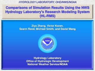
Hydrology Laboratory Research Modeling System (HL-RMS) Introduction:. Fekadu Moreda Presented to Mid-Atlantic River Forecasting Center February, 15, 2005. Office of Hydrologic Development National Weather Service National Oceanic and Atmospheric Administration. Over View.

E N D
Hydrology Laboratory Research Modeling System (HL-RMS) Introduction: Fekadu Moreda Presented to Mid-Atlantic River Forecasting Center February, 15, 2005 Office of Hydrologic Development National Weather Service National Oceanic and Atmospheric Administration
Over View • Historical Perspective • Motivation • Definition of a Distributed Hydrologic Model • Structure of HL-RMS and Components • Parameterization • Forcings (Precipitation, Temperature, Evaporation) • Case Study
(1) Historical Perspective • Rational formula • Unit Hydrograph • Event based model • Continuous simulation models • Semi-distributed models • Fully Distributed models
(2) Motivation for distributed Models • Availability of high resolution data: basin properties and /forcings • Better stream flow forecasting • River and flash flood forecasting, • Soil moisture products • Snow cover • Potential extension to environmental models • Non-point source pollution • Land-use change (can account for burn areas) • Erosion studies • Landslide/mudslide/soil strength applications • Land-atmosphere interactions for meteorological and climate applications • Groundwater recharge and contamination studies • Others
(3) Definition of a Distributed Hydrologic model -(informal definition) a model which accounts for the spatial variability of factors affecting runoff generation: • precipitation • temperature • terrain • soils • vegetation • land use • channel shape
Generic Modeling Steps Lumped Model Distributed Model Derive mean areal precipitation (MAP) Derive model element precipitation Compute model element runoff Compute basin runoff Lumped runoff and soil moisture states Distributed runoff and Soil moisture states Apply distributed routing model Apply unit hydrograph Discharge hydrograph at any model element Discharge hydrograph at the outlet
Hydrologic Modeling Approaches Distributed Lumped • Rainfall, properties averaged over basin • One rainfall/runoff model • Prediction at only one point • Rainfall, properties in each grid • Rainfall/runoff model in each grid • Prediction at many points
Hydrology LabDistributed Model(HL-Research Modeling System HL-RMS) • Modular, flexible modeling system • Gridded (or small basin) structure • Independent rain+melt calculations for each grid cell (SNOW-17) • Independent rainfall-runoff calculations for each grid cell • Sacramento Soil Moisture Accounting (SAC-SMA) • Continuous Antecedent Precipitation Index (CONT-API) • Grid to grid routing of runoff (kinematic) • Channel routing (kinematic & Muskingum-Cunge)
HL-RMS Elements The surface and base flow components for each grid is obtained from a SAC-SMA rainfall –runoff model
The API MODEL 1st Quadrant 4th Quadrant API AIXW.CWAPI Fg=CG(AIf-AICR) 1.0 AIXD.CDAPI Fg 0.5 AIXD 0.0 AI Fs FRSX AIXW AICR Fs=FRSX.CRAIF SMI/SMIX=1.0 =0.9 2nd Quadrant 3rd Quadrant AIf The surface and base flow components for each grid is obtained from a CONT-API rainfall –runoff model
SNOW-17 SNOW 17 model is used in each element
Distributed routing • Translates distributed runoff into distributed stream flow • With distributed routing, flow velocity in each element is dependent on flow level • Different flows (states) are computed for each element in a stream network. Unit graph only produces flows at basin outlets. • Commonly used approach: numerical solution to the 1-D equations for momentum and mass conservation 2. Lumped and distributed modeling
Components of HL-RMS (P, T) SNOW Model SNOW-17 rain+melt Surface Runoff SAC-SMA /CONT-API Hillslope routing Base flow Channel routing Stream Flow
(4) Parameterization • Basic watershed properties • SNOW-17 model parameters • Cont-API parameters • Routing parameters
(a) Basic watershed properties • Digital Elevation Model (DEM) • Available for each of RFC with 400m resolution. 4km resolution (HRAP) is used in HL-RMS • Directly used in the SNOW-17 model • Flow Direction and Accumulations are derived from DEM • Location of outlets (lat long HRAP) • Connectivity file – ASCII file
Connectivity of Pixels Basins in MARFC Saxton
(b) SNOW-17 Parameter Grids • Ongoing work to develop distributed snow parameters • Use of Elevation (DEM) at HRAP grid cell • The traditional snow depletion curve may be replaced by two methods. • i) Assuming SI=0 => for a given time step in a pixel this snow or no snow • ii) Assuming a 45 degree depletion line for each grid. Since the 4km grid is much smaller than a a basin scale, this method will assume uniform coverage and depletion in a pixel
(c) CONT –API Parameter Grids • A priori parameters for 11 parameters derived from lumped model • Use lumped model parameters for others • Use the Evaporation index only • No frozen ground option • Parameters can be replaced by a lumped value or adjusted by a factor
(d) Routing Parameter Grids • Hillslope routing parameter grids: Hillslope slope (Sh) Hillslope roughness (nh) Channel density (D) • Channel routing: Channel slope (Sc) Channel roughness(nc) Channel width and shape parameters (a, b) • -OR- Specific discharge (a) and shape parameter (b) from a discharge cross-sectional area relationship (a, b)
METHOD TO ESTIMATE CHANNEL ROUTING PARAMETERS • Momentum equation describing steady, uniform flow: • Q is flow [L3/T] • A is cross-section area [L2] Parameters a and b must be estimated for each model grid cell. Basic Idea: (1) Estimate channel parameters at basin outlet using USGS flow measurement data. (2) Estimate parameters in upstream cells using relationships from geomorphology and hydraulics. Two methods are being tested: 3. METHOD TO ESTIMATE CHANNEL ROUTING PARAMETERS 3. METHOD TO ESTIMATE CHANNEL ROUTING PARAMETERS • Momentum equation describing steady, uniform flow: • Q is flow [L3/T] • A is cross-section area [L2] • Momentum equation describing steady, uniform flow: • Q is flow [L3/T] • A is cross-section area [L2] Parameters a and b must be estimated for each model grid cell. Parameters a and b must be estimated for each model grid cell. Parameters a and b must be estimated for each model grid cell. Basic Idea: (1) Estimate channel parameters at basin outlet using USGS flow measurement data. (2) Estimate parameters in upstream cells using relationships from geomorphology and hydraulics. Two methods are being tested: Basic Idea: (1) Estimate channel parameters at basin outlet using USGS flow measurement data. (2) Estimate parameters in upstream cells using relationships from geomorphology and hydraulics. Two methods are being tested:
(Tokar and Johnson 1995) (Tokar and Johnson 1995) (Tokar and Johnson 1995) (Gorbunov 1971) Channel Shape Method: • Assume simple channel shape. (B = width, H = depth) • From USGS data, estimate α, β, and channel roughness (n) at the outlet • Using an empirical equation, estimate local parameter nc using channel slope (So) and drainage area (Fo) at the outlet. Estimate ni at upstream cells. • For a selected flow level at the outlet, estimate spatially variable ai values (for each cell i) using Qi and Ai estimates derived from geomorphological relationships (see below) • Assume β is spatially constant within a basin and compute ai and bi at each cell using ai b, and ni, • Channel Shape Method: • Assume simple channel shape. (B = width, H = depth) • From USGS data, estimate a, b, and channel roughness (n) at the outlet • Using an empirical equation, estimate local parameter nc using channel slope (So) and drainage area (Fo) at the outlet. Estimate ni at upstream cells. • For a selected flow level at the outlet, estimate spatially variable ai values (for each cell i) using Qi and Ai estimates derived from geomorphological relationships (see below) • Assume b is spatially constant within a basin and compute aiand bi at each cell using aib, and ni, • Rating Curve Method: • Determine ao and bo at the outlet directly from regression on the flow measurement data. • Using the same geomorphological relationships as in the channel shape method, equations for estimating ai and bi can be derived: • Geomorphological Assumptions: • On average, flow is a simple function of drainage area and downstream flow. Leopold (1994), Figure 5.7 suggests g may vary from 0.65 to 1 in different parts of the U.S. Results shown here use g = 1 and g = 0.8. • On average, cross-sectional area of flow can be related to stream order. Rl is Horton’s length ratio, k is stream order
(Tokar and Johnson 1995) (Gorbunov 1971) (Gorbunov 1971) Rating Curve Method: • Determine ao and bo at the outlet directly from regression on the flow measurement data. • Using the same geomorphological relationships as in the channel shape method, equations for estimating ai and bi can be derived: • Geomorphological Assumptions: • On average, flow is a simple function of drainage area and downstream flow. Leopold (1994), Figure 5.7 suggests g may vary from 0.65 to 1 in different parts of the U.S. Results shown here use g = 1 and g = 0.8. • On average, cross-sectional area of flow can be related to stream order. Rl is Horton’s length ratio, k is stream order
6) Forcings • Gridded Precipitation • Temperature • Evaporation
(a) Gridded precipitation • Gridded products archived: http://dipper.nws.noaa.gov/hdsb/data/nexrad/nexrad.html • -available products: • GAGEONLY • RMOSAIC • MPE (XMRG) • One file for one hour for the entire RFC
(b) Gridded Temperature • Gridded products archived are available: • Hydrometeorology group: David Kitzmiller • Use of the MAT for the basins to generate grid products • Requires • A program to generate grids • Basin definitions (connectivity file) • MAT for each basin • Elevation map • Regional lapse rate
(c) Gridded Evaporation • Evaporation is essential for CONT-API • Only the evaporation option is tested • For now we will use seasonal evaporations • Monthly adjustments are used • Maps are available in CAP (Calibration Assistant Program)
(7) Case study • Juniata River Basin (11 subbasins)
First HL-RMS Run for Juniata Williamsburg, Interior point Outlet, Juniata at Newport Saxton, Interior point - Model resolution 4km x 4km - Total number of pixels =497 - Watershed area = 8687 km2 - Model parameters = a priori - Channel parameters are derived from USGS measurements at New port.
Summary • Introduced distributed hydrologic modeling • Develop skill in handling distributed data, parameter, and output • Distributed model complements the existing operation • Opportunities in future to apply to small basins, interior points for flash flood