Download
1 / 32
320 likes | 335 Views
Data Converter Basics. Dr. Hossein Shamsi. Chapter 1. Sampling, Quantization, Reconstruction. The Data Conversion Problem. Real world signals Continuous time, continuous amplitude Digital abstraction (concept) Discrete time, discrete amplitude. Overview. Uniform Sampling and Quantization.

E N D
Data Converter Basics Dr. Hossein Shamsi
Chapter 1 Sampling, Quantization, Reconstruction
The Data Conversion Problem • Real world signals • Continuous time, continuous amplitude • Digital abstraction (concept) • Discrete time, discrete amplitude
Uniform Sampling and Quantization • Most common way of performing A/D conversion • Sample signal uniformly in time • Quantize signal uniformly in amplitude • Key questions • How fast do we need to sample? • Must avoid "aliasing“ • How much "noise" is added due to amplitude quantization?
Sampling Theorem • In order to prevent aliasing, we need • The sampling rate fs=2·fsig,max is called the Nyquist rate • Two possibilities • Sample fast enough to cover all spectral components, including "parasitic" ones outside band of interest • Limit fsig,max through filtering
Practical Anti-Alias Filter • Need to sample faster than Nyquist rate to get good attenuation • Oversampling
How much Oversampling? • Can tradeoff sampling speed against filter order • In high speed converters, making fs/fsig,max>10 is usually impossible or too costly • Means that we need fairly high order filters
Classes of Sampling • Nyquist-rate sampling (fs > 2·fsig,max) • Nyquist data converters • In practice always slightly oversampled • Oversampling (fs >> 2·fsig,max) • Oversampled data converters • Anti-alias filtering is often trivial • Oversampling also helps reduce "quantization noise" • More later • Undersampling, subsampling (fs < 2·fsig,max) • Exploit aliasing to mix RF/IF signals down to baseband
Quantization of an Analog Signal • Quantization step Δ • Quantization error has sawtooth shape • Bounded by –Δ/2, + Δ /2 • Ideally • Infinite input range and infinite number of quantization levels • In practice • Finite input range and finite number of quantization levels • Output is a digital word (not an analog voltage)
Conceptual Model of a Quantizer • Encoding block determines how quantized levels are mapped into digital codes • Note that this model is not meant to represent an actual hardware implementation • Its purpose is to show that quantization and encoding are conceptually separate operations • Changing the encoding of a quantizer has no interesting implications on its function or performance
Encoding Example for a B-Bit Quantizer • Example: B=3 • 23=8 distinct output codes • Diagram on the left shows "straight-binary encoding“ • See e.g. Analog Devices "MT-009: Data Converter Codes" for other encoding schemes • http://www.analog.com/en/content/0,2886,760%255F788%255F91285,000 • Quantization error grows out of bounds beyond code boundaries • We define the full scale range (FSR) as the maximum input range that satisfies |eq| ≤ Δ/2 • Implies that FSR=2B·Δ
Nomenclature (فهرست نام ها) • Overloading - Occurs when an input outside the FSR is applied • Transition level – Input value at the transition between two codes. By standard convention, the transition level T(k) lies between codes k-1 and k • Code width – The difference between adjacent transition levels. By standard convention, the code width W(k)=T(k+1)-T(k) • Note that the code width of the first and last code (000 and 111 on previous slide) is undefined • LSB size (or width) – synonymous with code width Δ
Implementation Specific Technicalities • So far, we avoided specifying the absolute location of the code range with respect to "zero" input • The zero input location depends on the particular implementation of the quantizer • Bipolar input, mid-rise or mid-tread quantizer • Unipolar input • The next slide shows the case with • Bipolar input • The quantizer accepts positive and negative inputs • Represents common case of a differential circuit • Mid-rise characteristic • The center of the transfer function (zero), coincides with a transition level
Bipolar Mid-Rise Quantizer • Nothing new here..
Bipolar Mid-Tread Quantizer • In theory, less sensitive to small disturbance around zero • In practice, offsets larger than Δ/2 (due to device mismatch) often make this argument irrelevant • Asymmetric full-scale range, unless we use odd number of codes
Unipolar Quantizer • Usually define origin where first code and straight line fit intersect • Otherwise, there would be a systematic offset • Usable range is reduced by Δ/2 below zero
Effect of Quantization Error on Signal • Two aspects • How much noise power does quantization add to samples? • How is this noise power distributed in frequency? • Quantization error is a deterministic function of the signal • Should be able answer above questions using a deterministic analysis • But, unfortunately, such an analysis strongly depends on the chosen signal and can be very complex • Strategy • Build basic intuition using simple deterministic signals • Next, abandon idea of deterministic representation and revert to a "general" statistical model (to be used with caution!)
Ramp Input • Applying a ramp signal (periodic sawtooth) at the input of the quantizer gives the following time domain waveform for eq • What is the average power of this waveform? • Integrate over one period
Sine Wave Input • Integration is not straightforward...
Quantization Error Histogram • Sinusoidal input signal with fsig=101Hz, sampled at fs=1000Hz • 8-bit Quantizer • Distribution is "almost" uniform • Can approximate average power by integrating uniform distribution
Statistical Model of Quantization Error • Assumption: eq(x) has a uniform probability density • This approximation holds reasonably well in practice when • Signal spans large number of quantization steps • Signal is "sufficiently active" • Quantizer does not overload
Reality Check (1) • Sine wave example, but now fsig/fs=100/1000 • What's going on here?
Analysis (1) • Sampled signal is repetitive and has only a few distinct values • This also means that the Quantizer generates only a few distinct values of eq; not a uniform distribution
Analysis (2) • Signal repeats every m samples, where m is the smallest integer that satisfies • This means that eq(n) has at best 10 distinct values, even if we take many more samples
Signal-to-Quantization-Noise Ratio • Assuming uniform distribution of eq and a full-scale sinusoidal input, we have
Quantization Noise Spectrum (1) • How is the quantization noise power distributed in frequency? • First think about applying a sine wave to a quantizer, without sampling (output is continuous time) • Quantization results in an "infinite" number of harmonics
Quantization Noise Spectrum (2) • Now sample the signal at the output • All harmonics (an "infinite" number of them) will alias into band from 0 to fs/2 • Quantization noise spectrum becomes "white” • Interchanging sampling and quantization won’t change this situation results in an "infinite" number of harmonics
Quantization Noise Spectrum (3) • Can show that the quantization noise power is indeed distributed (approximately) uniformly in frequency • Again, this is provided that the quantization error is "sufficiently random" “one-sided spectrum”