Download
1 / 28
330 likes | 664 Views
Data Compression Basics. Main motivation: The reduction of data storage and transmission bandwidth requirements.

E N D
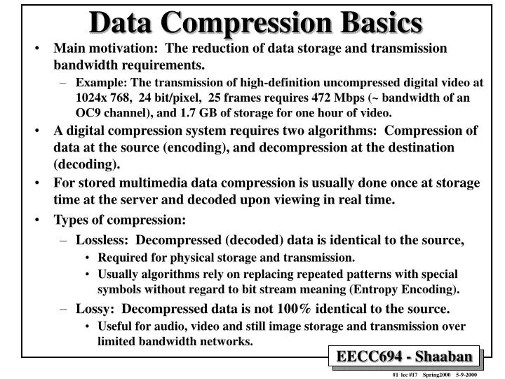
Data Compression Basics • Main motivation: The reduction of data storage and transmission bandwidth requirements. • Example: The transmission of high-definition uncompressed digital video at 1024x 768, 24 bit/pixel, 25 frames requires 472 Mbps (~ bandwidth of an OC9 channel), and 1.7 GB of storage for one hour of video. • A digital compression system requires two algorithms: Compression of data at the source (encoding), and decompression at the destination (decoding). • For stored multimedia data compression is usually done once at storage time at the server and decoded upon viewing in real time. • Types of compression: • Lossless: Decompressed (decoded) data is identical to the source, • Required for physical storage and transmission. • Usually algorithms rely on replacing repeated patterns with special symbols without regard to bit stream meaning (Entropy Encoding). • Lossy: Decompressed data is not 100% identical to the source. • Useful for audio, video and still image storage and transmission over limited bandwidth networks.
From Information Theory: • Information is quantifiable as: Average Information = - log2 (prob. of occurrence) • For English: -log(1/26) = 4.7 • Why is information stored using 8 bits? • Extended ASCII has 256 symbols. • This is a non-optimal encoding since it assumes an even distribution of probabilities for all symbols.
Entropy • For a statistically independent source, the extension of the previous definition of average information, is called Entropy H(s): • It can be seen as the probability-weighted average of the information associated with a message. • It can be interpreted much like it is in thermodynamics, the higher the entropy, the greater its lack of predictability. • Hence, more information is conveyed in it. • This leads to the relationship: Average Length >= H(S)
Entropy (continued) Example: Assume a three symbol alphabet {A, B, C} with symbol probabilities given as: P(A) = 0.5 P(B) = 0.33 P(C) = 0.167 • In this case, Entropy: H(S) = 1.45 bits • If P(A) = P(B) = P(C) = 1/3 • Then H(S) = 1.58 bits • This demonstrates that sources which have symbols with high probability should be represented by fewer bits. • In reality, information is not always coded using the theoretic entropy (optimal encoding). • The excess is defined as redundancy and is seen in character repetition, character distribution, usage patterns, and from positional relativeness.
Lossless Compression • All lossless compression methods work by identifying some aspect of non-randomness (redundancy) in the input data, and by representing that non-random data in a more efficient way. • There are at least two ways that data can be non-random. • Some symbols may be used more often than others, for example in English text where spaces and the letter E are far more common than dashes and the letter Z. • There may also be patterns within the data, combinations of certain symbols that appear more often than other combinations. If a compression method was able to identify that repeating pattern, it could represent it in some more efficient way. • Examples: • Run-Length Encoding (RLE). • Huffman Coding. • Arithmetic coding. • Shannon-Fano Coding. • LZ78, LZH, LZW, … etc.
Lossless Compression Example: Run-Length Encoding (RLE) • Works by representing runs of a repeated symbol by a count-symbol combination. • Run-length encoding may be used as one of the steps of more elaborate compression schemes. • Example: • The input string: aaaaaaabbaaabbbbccccc • Becomes: <esc>7abb<esc>3a<esc>4b<esc>5c • 7 bytes are saved. • Effective only for runs greater than 3 bytes. • Applications are limited.
Lossless Compression Example: Shannon-Fano Coding • Number of bits required to represent a code is proportional to the probability of the code. • Resulting Codes are uniquely decodable. They obey a prefix property. • Compressor requires two passes or a priori knowledge of the source. • Decompressor requires a priori knowledge or communication from compressor. • Develop a probability for the entire alphabet, such that each symbol’s relative frequency of appearance is know. • Sort the symbols in descending frequency order. • Divide the table in two, such that the sum of the probabilities in both tables is relatively equal. • Assign 0 as the first bit for all the symbols in the top half of the table and assign a 1 as the first bit for all the symbols in the lower half. (Each bit assignment forms a bifurcation in the binary tree.) • Repeat the last two steps until each symbol is uniquely specified.
Shannon-Fano Coding Example (Continued) Symbol Encoding Binary Tree forming code table.
Huffman Coding • Similar to Shannon-Fano in that it represents a code proportional to its probability. • Major difference: Bottom Up approach. • Codes are uniquely decodable. They obey a prefix property. • Develop a probability for the entire alphabet, such that each symbol’s relative frequency of appearance is know. • Sort the symbols, representing nodes of a binary tree, in prob. order • Combine the probabilities of the two smallest nodes and create/add a new node, with its probability equal to this sum, to the list of available nodes. • Label the two leaf nodes of those just combined as 0 and 1 respectively, and remove them from the list of available nodes. • Repeat this process until a binary tree is formed by utilizing all of the nodes.
Huffman Coding Example Symbol Encoding Binary Tree forming Huffman code table.
Lossy Compression • Takes advantage of additional properties of the data to produce more compression than that possible from using redundancy information alone. • Usually involves a series of compression algorithm-specific transformations to the data, possibly from one domain to another (e.g to frequency domain in Fourier Transform), without storing all the resulting transformation terms and thus losing some of the information contained. • Examples: • Differential Encoding: Store the difference between consecutive data samples using a limited number of bits. • Discrete Cosine Transform (DCT): Applied to image data. • Vector Quantization. • JPEG (Joint Photographic Experts Group). • MPEG (Motion Picture Experts Group).
Lossy Compression Example: Vector Quantization Image is divided into fixed-size blocks A code book is constructed which has indexed image blocks of the same size representing types of image blocks. Instead of transmitting the actual image: The code book is transmitted + The corresponding block index from the code book or the the closest match bloc index is transmitted. Encoded Image Transmitted
Transform Coding Lossy Image Compression methods • Transform: Applies an invertible linear coordinate transformation to the image. • Quantize: Replaces the transform coefficients with lower-precision approximations which can be coded in a more compact form. • Encode: Replaces the stream of small integers with some more efficient alphabet of variable-length characters. • In this alphabet the frequently occurring letters are represented more compactly than rare letters. • This lossy compression scheme becomes lossless if the quantize step is omitted: • Because the quantize step may discard or reduce the precision of unnecessary coefficients leaving important features to be encoded. • Example: Joint Photographic Experts Group (JPEG).
Transform Quantize Encode JPEG Lossy Sequential Mode Lossy Compression Example: Joint Photographic Experts Group (JPEG) • JPEG Compression Ratios: • 30:1 to 50:1 compression is possible with small to moderate defects. • 100:1 compression is quite feasible for very-low-quality purposes .
JPEG Steps • Block Preparation: From RGB to Y, I, Q planes (lossy). • Transform: Two-dimensional Discrete Cosine Transform (DCT) on 8x8 blocks. • Quantization: Compute Quantized DCT Coefficients (lossy). • Encoding of Quantized Coefficients : • Zigzag Scan. • Differential Pulse Code Modulation (DPCM) on DC component. • Run Length Encoding (RLE) on AC Components. • Entropy Coding: Huffman or Arithmetic.
Compression: Transform Quantize Encode JPEG Overview Block Preparation Transform Quantize Decompression: Reverse the order Encode
JPEG: Block Preparation RGB Input Data After Block Preparation • Input image: 640 x 480 RGB (24 bits/pixel) transformed to three planes: • Y: (640 x 480, 8-bit/pixel) Luminance (brightness) plane. • I, Q: (320 X 240 8-bits/pixel) Chrominance (color) planes.
Discrete Cosine Transform (DCT) A transformation from spatial domain to frequency domain (similar to FFT) Definition of 8-point DCT: F[0,0] is the DC component and other F[u,v] define AC components of DCT
The 64 (8 x 8) DCT Basis Functions u DC Component v
8x8 DCT Example or v or u DC Component Original values of an 8x8 block (in spatial domain) Corresponding DCT coefficients (in frequency domain)
JPEG: Computation of Quantized DCT Coefficients q(u,v) Uniform quantization: Divide by constant N and round result. In JPEG, each DCT F[u,v] is divided by a constant q(u,v). The table of q(u,v) is called quantization table. F[u,v] Rounded F[u,v]/ q(u,v)
JPEG: Transmission Order of Quantized ValuesZigzag Scan Maps an 8x8 block into a 1 x 64 vector Zigzag pattern group low frequency coefficients in top of vector.
Encoding of Quantized DCT Coefficients • DC Components: • DC component of a block is large and varied, but often close to the DC value of the previous block. • Encode the difference of DC component from previous 8x8 blocks using Differential Pulse Code Modulation (DPCM). • AC components: • The 1x64 vector has lots of zeros in it. • Using RLE, encode as (skip, value) pairs, where skip is the number of zeros and value is the next non-zero component. • Send (0,0) as end-of-block value.
JPEG: Entropy Coding • Categorize DC values into SSS (number of bits needed to represent) and actual bits. -------------------- Value SSS 0 0 -1,1 1 -3,-2,2,3 2 -7..-4,4..7 3 -------------------- • Example: if DC value is 4, 3 bits are needed. • Send off SSS as Huffman symbol, followed by actual 3 bits. • For AC components (skip, value), encode the composite symbol (skip,SSS) using the Huffman coding. • Huffman Tables can be custom (sent in header) or default.
Compression Ratio: 12.3 Original Image Compression Ratio: 7.7 Compression Ratio: 33.9 Compression Ratio: 60.1 Quantization Table Used Compressed Image JPEG Example Produced using the interactive JPEG Java applet at: http://www.cs.sfu.ca/undergrad/CourseMaterials/CMPT365/material/misc/interactive_jpeg/Ijpeg.html