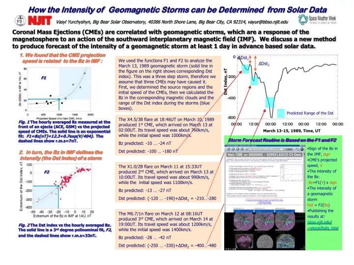
How the Intensity of Geomagnetic Storms can be Determined from Solar Data

1. How the Intensity of Geomagnetic Storms can be Determined from Solar Data Vasyl Yurchyshyn, Big Bear Solar Observatory, 40386 North Shore Lane, Big Bear City, CA 92314, vayur@bbso.njit.edu Coronal Mass Ejections (CMEs) are correlated with geomagnetic storms, which are a response of the magnetosphere to an action of the southward interplanetary magnetic field (IMF). We discuss a new method to produce forecast of the intensity of a geomagnetic storm at least 1 day in advance based solar data. 1. We found that the CME projection speed is related to the Bz in IMF : ΔDst1 We used the functions F1 and F2 to analyze the March 13, 1989 geomagnetic storm (solid line in the figure on the right shows corresponding Dst index). This was a three step storm, therefore we assume that three CMEs may have caused it. First, we determined the source regions and the initial speed of the CMEs, then we calculated the Bz in the corresponding magnetic clouds and the range of the Dst index during the storms (blue boxes). ΔDst2 F1 Dst Index, nT Predicted Range of the Dst The X4.5/3B flare at 18:46UT on March 10, 1989 produced 1st CME, which arrived on March 13 at 02:00UT. Its travel speed was about 760km/s, while the initial speed was 1000km/s. Bz predicted: -10 … -24 nT Dst predicted: -100 … -180 nT Fig. 1 The hourly averaged Bz measured at the front of an ejecta (ACE, GSM) vs the projected speed of CMEs. The solid line is an exponential fit: F1=Bz[nT]=12.3+0.7exp(V/404). The dashed lines show r.m.s=7nT. March 13-15, 1989, Time, UT Storm Forecast Routine is Based on the F1 and F2 •Sign of the Bz in the IMF, sign •CME’s projected speed, V •The intensity of the Bz: Bz=F1(V) x sign •The intensity of a geomagnetic storm Dst = F2(Bz) •Publishing the results at: bbso.njit.edu/ ~vayur/halo_cme 2. In turn, the Bz in IMF defines the intensity (the Dst Index) of a storm The X1.0/2B flare on March 11 at 15:33UT produced 2nd CME, which arrived on March 13 at 10:00UT. Its travel speed was about 990km/s, while the initial speed was 1100km/s. Bz predicted: -13 … -27 nT Dst predicted: (-120 … -190)+ΔDst1 = -210…-280 F2 The M6.7/1n flare on March 12 at 08:16UT produced 3rd CME, which arrived on March 14 at 19:00UT. Its travel speed was about 1200km/s, while the initial speed was 1400km/s. Bz predicted: -28 … -42 nT Dst predicted: (-250 … -330)+ΔDst2 = -400…-480 Fig. 2 The Dst index vs the hourly averaged Bz. The solid line is a 3rd degree polinominal fit, F2, and the dashed lines show r.m.s=33nT.