Download
1 / 31
320 likes | 458 Views
------Using GIS--. Introduction to GIS. Raster Query Map Calculation Zonal statistics Terrain functions Viewshed (Visibility) analysis. Introduction to Raster Spatial Analysis. ------Using GIS--. Introduction to GIS. Raster data-A Refresher. Grid Elements Extent # rows

E N D
------Using GIS-- Introduction to GIS • Raster Query • Map Calculation • Zonal statistics • Terrain functions • Viewshed (Visibility) analysis Introduction to Raster Spatial Analysis
------Using GIS-- Introduction to GIS Raster data-A Refresher Grid Elements Extent # rows # columns Coordinates Origin Resolution Grid cell
------Using GIS-- Introduction to GIS Raster Overlay Queries The raster data model performs overlay operations more efficiently than the vector model. Raster cells have a one-to-one relationship between layers Raster overlay queries involve the combining of two or more separate thematic layers to identify relationships between them such as: Areas that meet criteria from each layer Query example: [elevation > 2500] AND [Slope>20]
------Using GIS-- Introduction to GIS Overlay Calculations Map algebra can be performed to identify relationships between layers, or to derive indices that describe phenomena Map calculations create a new layer Calculation example: (Soil_depth_1990) – (Soil_depth_2000)=loss in soil between 1990 and 2000
------Using GIS-- Introduction to GIS Map Query Examples Single layer numeric example: elevation > 2000 ft
Map Query Examples Results in a binary True/False layer
------Using GIS-- Introduction to GIS Map Query Examples 11 12 13 14 17 Multi-criteria, single layer, categorical map query: looking for all developed land use types, using attribute codes (11, 12, 13, 14, 17) and ‘OR’ Vertical lines mean OR
------Using GIS-- Introduction to GIS Map Query Examples Results in a 1/0 binary layer, showing urbanized areas
------Using GIS-- Introduction to GIS Map Query Examples One can then convert this to a vector shapefile or feature class
------Using GIS-- Map Query: 3-layer Examples Let’s say we want to identify potential habitat for a rare plant that grows at higher elevation, on steeper slopes and in coniferous forest Multi-layer queries uses criteria across two or more layers; in this case we’ll query land use (categorical), elevation (number) and slope (number)
------Using GIS-- Map Query Examples First we would generate a slope map from out Digital Elevation Model by going to Surface>>Derive Slope
------Using GIS-- Introduction to GIS Map Query Examples Let’s say our criteria are elevation >800, slope >20% and land use category= coniferous forest (42)
------Using GIS-- Introduction to GIS Map Query Examples Again we end up with a 1/0 binomial query layer
------Using GIS-- Map Calculation We can also run calculations between layers: here we’ll multiply the k factor (soil erodability factor) by slope; let’s just imagine this will yield a more accurate and spatially explicit index of erodability that factors in slope at each pixel
------Using GIS-- Introduction to GIS Map Calculation Now we simply type in the equation and a new grid is created that solves that equation
------Using GIS-- Map Calculation The darker areas are those with both steep slope and erodable soils. This has the advantage over map query in that we now have a continuous index of values, rather than just a “true” “false” dichotomy
------Using GIS-- Map Calculation and Query We could then, for instance, run a map query to find areas that have high erodability factors and urban land use.
------Using GIS-- Introduction to GIS Zonal Statistics Now, say we had a proposed subdivision map (this one is made up). We could overlay it on our new index layer and figure out which proposed subdivisions are problematic
------Using GIS-- Introduction to GIS Zonal Statistics Using Zonal Statistics we could summarize the mean, max or sum of the soil index for each of those units, even though one is grid and one is polygon. Here we summarize the erodability index by subdivision zones.
------Using GIS-- Summary by Zone Polygon layer with zones Unique ID for polygons This will create a DBF table that summarizes the pixel values by mean, median, max, min, etc., of all the pixels falling within a given polygon. Each row represent a polygon and each column represents a different summary statistic This joins the DBF table to the polygon layer Statistic by which your data will be charted
------Using GIS-- Summary by Zone It gives us a DBF table with values of mean, max, min, stdv, etc. in the table, plus a chart summarizing the means;
------Using GIS-- Summary by Zone Now we can plot out the subdivision boundaries (zones) by a soil erosion statistic. In this case, clearly the most meaningful one is the mean of the soil erosion statistic. This represent the mean value, by polygon, of all the soil erosion pixels underlaying that polygon
------Using GIS-- Raster terrain functions in ArcGIS ArcGIS allows you to take a digital elevation model (DEM) and derive: Hillshade Aspect Slope Contours
------Using GIS-- Raster terrain functions DEM + Hillshade = Hillshaded + =
------Using GIS-- Raster terrain functions in AV This is done by making a hillshade using Spatial analyst, putting the hillshade “under” the DEM in the TOC and making the DEM transparent
------Using GIS-- Raster terrain functions in Arc GIS Slope: Contours: Aspect:
Viewshed analysis (Visibility analysis) This is a multi-layer function that analyzes visibility based on terrain. It requires a grid terrain layer and a point layer and produces a visibility grid layer that tells you where the feature can be seen from, or alternately, what areas someone standing at that feature could see (remember, line of sight is two way). If there are more than one point feature, then each grid cell tells you how many of the point features can be seen from a given point.
Introduction to GIS Viewshed analysis Let’s say we’re local planners who are considering putting in a new waste treatment facility in valley where the vacation homes of five rich and powerful Hollywood executives are located. We want it in a place that won’t ruin anyone’s views, since they comprise 95% of the local tax base. So we geocode the house locations, overlay them on a high-resolution digital elevation model and run a viewshed analysis This generates a grid with three values, representing how many houses can see a given pixel
Viewshed analysis This is done in ArcGIS, but can also be done in ArcView. Red represents areas that can be seen by 1 house, blue by 2 or more
Viewshed analysis In order to compare the visability of several facilities, separate viewshed analyses need to be done for each feature. In the next example we will look at three candidate sites for a communications tower. Each will produce a visability grid. This grid can then be superimposed on a layer showing residential areas. Since each grid will belong to a different tower, we can tell which tower will be most viewable from the residential areas through simple overlay analysis.
Introduction to GIS Viewshed analysis In this case, red is for tower 1, blue for 2 and green for 3