Download
1 / 46
460 likes | 530 Views
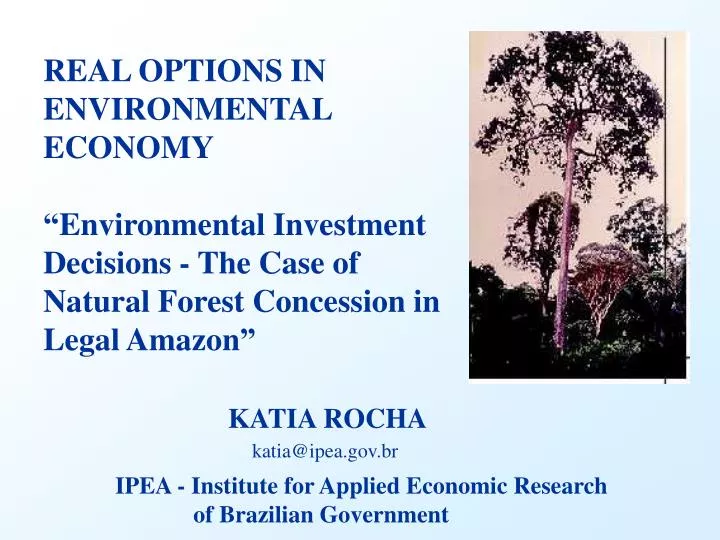
REAL OPTIONS IN ENVIRONMENTAL ECONOMY “Environmental Investment Decisions - The Case of Natural Forest Concession in Legal Amazon”. KATIA ROCHA. katia@ipea.gov.br. IPEA - Institute for Applied Economic Research of Brazilian Government. Forest Lease in Legal Amazon - Overview.

E N D
REAL OPTIONS IN ENVIRONMENTAL ECONOMY “Environmental Investment Decisions - The Case of Natural Forest Concession in Legal Amazon” KATIA ROCHA katia@ipea.gov.br IPEA - Institute for Applied Economic Research of Brazilian Government
Forest Lease in Legal Amazon - Overview • Brazilian Government : • Planning to implement • Natural Forest concession • in Legal Amazon • Legal Amazon : 500 millions hectares • Volume estimated : 60 billions m3 of wood • Annual production : 25 millions m3 of wood • Area for logging : 3% of Legal Amazon • Discussion : Increasing logging area up to 12 % • Legal process : Analyzed by the Brazilian congress.
Forest Lease in Legal Amazon - Overview • Participation on • international market: • 4 % of global exportations • Expansion over next decade • - gradual exhaustion of the Asian forestry resources - • Regulatory Policies : • the minimum inventory held in the lease area, • the maximum extraction rates allowed, • the use of environmental handling techniques
Environmental and Economical Issues • Concern : Economic Market Value of concession • Focus on Expected Cash Flows and Option Values • Environmental commodities has been suggested : • Forest Products • Harvest allowances - analogy to the “pollution allowances” • used in USA. • These allowances add value and options to the leaseonwer • Real Options can quantify social benefits coming from: • kidnapping of carbon • contribution to global climatic stability • water balance maintenance • preservation of biodiversity
Forest Lease as Real Option • Forest Lease is a Capital Investment Opportunity • Long time horizon - usually 30 years • High uncertainty about timber prices and inventory • Option : Right but not the obligation to proceed the harvest • Decisions: • When management should proceed the harvest ? • What is the optimal cutting rate policy? • Harvest decision is an instantaneous irreversible decision
Real Options on Renewable Resources -Literature- • Robert Pindyck (1984) • “Uncertainty in the Theory of Renewable Resources Markets” • Review of Economic Studies • Deterministic Prices and Stochastic Inventories • Price is function of aggregate extraction rate • Extraction Cost is a convex function of inventory • Inventory uncertainty reduces the lease value
Real Options on Renewable Resources -Literature- • Morck, Schwartz and Stangeland (1989) • “The Valuation of Forestry Resources under • Stochastic Prices and Inventories” • The Case of a White Pine Forest Lease in Alberta, Canada • Journal Financial and Quantitative Analysis • Stochastic Prices and Inventories • Price is uncorrelated to extraction rate or inventory • -small firm assumption- • Extraction Cost is quadratic function • Price uncertainty increases the lease value
Introduction to the Model • The present model is similar to Morck, Schwartz and Stangeland (1989) with slightly modification : • Comparisons between ROT and NPV are performed • Regulation Policies are included • Uncertainty over Initial Inventory - use of spatial econometric models - • Extraction cost is a linear function - realistic assumption • Further work - to model changes in timber price as a Mean-Reverting Process - standard for commodities
Formulating a Profit Maximization Inter-temporal Problem • ROT : inter-temporal maximization procedure under • uncertainty considering the options available to managers • Maximization tool : • Bellman´s Equation - Stochastic Dynamic Programming • split the decision sequence into two parts : Today Future expectations over all the future profits throughout the lifetime of the lease - continuation value - + Lease = Value immediate profit • Optimal action today is the one that maximizes the Value
Bellman´s Equation - Stochastic Dynamic Programming - 1 ) 2 ) Although 1 < 2 we have to use the expectations about the future. Therefore alternative 1 is the correct optimization procedure
Future Outcomes Comparing Optimization Procedure Future Outcomes Procedure 2 Procedure 1 prob = 0.5 A C prob = 0.5 q* qA* q q prob = 0.5 B prob = 0.5 D qB* q* q q Procedure 2 Procedure 1 > Max = (A+B). 1/2 Max = (C+D). 1/2 Optimal control DOES NOT exist Optimal control EXIST - q*
Option Premium • Management Decisions / Flexibilities : • “When to harvest ?” Option to Delay or Defer • “How much to harvest ?” Option to Expand or Contract • These flexibilities add an extra Value - Option Premium - • to the Lease. • Lease = NPV + Option Premium • ( Real Option Value )
Price and Inventory Uncertainties • 1 - The market price of timber: • “How the prices will be on the next decade or year ?” • 2 - The amount of timber inventory in the leasehold: • “How the timber inventory will grow in the lease area? Fast or Low?” • Loss of timber inventory : burnings, • limitations on cutting valuable species • Increase of timber inventory: discovery of new or valuable species • The best you can do is to add some uncertainty • to your forecast on timber price and inventory time • evolution processes {
Timber Prices • Wood price time series data : • Brazilian logs of medium value • Hardwood logs from Malaysia • (International Financial Statistics - IMF) • Both data present similar volatility 30 % p.a.
Hardwood Log Prices Price (jan ‘77 / jan ‘99) - $/m3 - in real prices of ‘95 Mean Reverting Process appears to be a good guess
USA Lumber X Malaysia Hardwood Price (jan ‘82 / apr ‘00) - $/m3 - in real prices of ‘95 Similar Pattern for US Lumber and Malaysia Hardwood Hardwood Conv.Yield could be approximated by Lumber Conv. Yield
Timber Price as a Stochastic Process. • Basic approach is to use Stochastic Differential Equations • - SDE • We use the standard Geometric Brownian Motion (GBM) : dP = changes in price P = Timber Price ($/m3) mP = average growth rate in % of price (% p.a.) sP =volatility parameter in % of price (% p.a.) Percentage changes in prices (dP/P) are normally distributed with mean mP t, and variance sP2 t. Variance grows as time passes by : Non-Stationary Process
Timber Inventory as a Stochastic Process • We use the standard Stochastic Differential Equation • from the population ecology literature dI = changes in Inventory I = Inventory of Timber in the leasehold (m3/ha) mI = average growth rate in % of timber inventory held (% p.a.) sI = volatility parameter in % of timber inventory held (% p.a.) q* = quantity of timber produced (m3/ha.year) q* = control variable that will be managed optimally
Mathematical Formulation for the Lease Value • Lease value is calculated by maximizing the expected • profit function throughout the lifetime of the lease Revenues Costs Discount Factor P = Timber Price q* = quantity of timber produced T = Lifetime of the lease C (q*) = cost function r = risk-free interest rate
Contingent Claims Approach • The Lease Value can be viewed as a Contingent Claim • on the underlying timber • Dynamic Programming with risk-neutral drift (r-k) discounting • by the risk-free rate Contingent Claims Approach • Continuos time finance assumptions : • 1 - There are futures markets for timber • - Forest Products on CME - Futures and Options on Lumber - • 2 - The convenience yield (k) is proportional • to the spot price of timber. • Convenience yield can be calculated using the • relationship between future price and spot price :
Contingent Claims Approach • Set up an instantaneous riskless portfolio using hedge • hedge : long and short positions over the underlying variable ( timber price) The hedge eliminates all market risk associated to timber price Market risk associated to stochastic changes in inventory is not appraised by the market. Risk is uncorrelated with market.Risk premium is zero • The riskless portfolio must earn the risk-free rate (r) to avoid arbitrage possibilities.
Lease Value Differential Equation • After application of Ito´s Lemma , the Lease Value -F(P,I,t) • follows the Partial Differential Equation (PDE) of • parabolic type in two dimensions (P & I) : subject to the appropriated boundary conditions “explained next” • Similar to B&S equation except by the terms in red • Analytical solution are rare • Numerical solution is always available • We use Finite Difference Method
Boundary Conditions and Constraints • F( P , I , t = T ) = 0 Null value at the expiration • F ( P = 0 , I , t ) = 0 Null value if price drops to zero • F( P , I = 0 , t ) = 0 Null value if the timber is over • For very high prices the value is • proportional to the inventory held • Reflector barrier due to the • geographic limitation • 0 < q*(P,I,t) < qmax Constraint on production capacity • q ( P , I < Imin , t ) = 0 Regulatory policy • bellow a certain level of inventory (Imin) the harvest is not allowed
Lease Value using NPV • Traditional Capital Budgeting (NPV): Free Cash Flows = Revenues - Costs , if FCF > 0 , if FCF < 0 subject to the constraint : • q( P , I < Imin , t ) = 0 Regulatory policy
Price uncertainty sensitivity analysison Lease Value ($/ha) at t = 0 (T=30) F PP > 0 Option or Lease Value FPP.P 2 Higher price uncertainty increase the Lease Value
Boundary Condition Effect (Price) Parallel Lines Equal derivatives F (P = 0) = 0 P = 0 P =
Inventory uncertainty sensitivity analysison Lease Value ($/ha) at t = 0 (T=30) Region A F II > 0 Region B F II < 0 NPV = 0 Option or Lease Value FII.I 2 Min. Inventory held 12.5 Inventory uncertainty produces different effects on the Lease value
Boundary Condition Effect (Inventory) NPV = 0 FI = 0 F (I = 0) = 0 Equal derivatives I = 0 I =
ROT & NPV outcomes Lease Value ($/ha) at t = 0 , for I = 25m3/ha and T = 30 years ROT +103 % NPV +96 % +115 %
Effect of Regulatory policy on Lease Value ($/ha) at t = 0 (T=30) +69 % +34 % Base Case Lease Value increases as Regulation becomes less intense
Interest rate sensitivity analysis on Lease Value ($/ha) at t = 0 (T=30) +112 % +57 % Base Case
Optimal cutting rate policy Cutting rate policy q* at t = 0, T=30 , for Total Cost = $12/m3 qmax P* = $14 r = 10 % p.a. P* = $12 r = 5 % p.a. P* = $16 r = 15 % p.a. Threshold - P* - increases as interest rate increases NPV rule : Static Threshold P* = Total Cost = $12
Concluding Remarks The application of ROT instead of NPV leads to : • Higher Values • Lease Value is 100 % higher for the base case • Different Thresholds • Threshold P* for harvest varies by an amount of 15 % relative to interest rate. NPV produces static Threshold (Costs) • Analysis about the Regulatory Policy • Reducing the regulatory limit in 50 % , leads to an increases • of 34% in the Lease value. NPV is not able to quantify this change
Numerical Techniques • Stochastic Optimization Problems can be solved by : • Simulation Processes : • Monte Carlo simulation with Optimization Method • Lattice Methods : • Binomial Method • Trinomial Method • Solving the Partial Differential Equation : • Analytical Solutions : Black & Scholes • Numerical Solutions : Finite Difference Method
Finite Difference Method • Implicit form : • The PDE can be solved indirectly by solving a system • of simultaneous linear equations • Convergence is always assured • Explicit form : • The PDE can be solved directly using the appropriated • boundary conditions and proceeding backward in time • through small intervals until find the optimal path • q*(P,I,t) to every t. • Convergence is assured for specifics size of increments • - interval length -
Finite Difference - Explicit Method • It consists of transforming the continuos domain of P, I • and t (state variables) by a network or mesh of discrete • points. • The PDE is converted into a set of finite difference • equations • Each unknown value is function of known values of the • subsequent period - backward procedure • unknown value t known values t+1 • The function represents weights and acts as “probabilities” Function “probabilities”
Finite Difference - Explicit Method . . . known values F( P , I , t ) = F( iDP, jDI , nDt ) i p- p0 p+ P = i DP Grid . . { DP ? . . . unknown value interval length for P . . “probabilities” { { j Dt DI t I = j DI interval length for I interval length for t
Discretization Process • Discretization to Lease Value : • F( P , I , t ) = F( iDP, jDI , nDt ) = F i,j,t • Partial derivatives are approximated by following • difference equations : • FPP = [ F i+1,j , t+1 - 2F i,j,t+1 + F i-1,j,t+1 ] / (DP)2 ; • FP = [ F i+1,j,t+1- F i-1,j,t+1 ] / 2DP ;central difference • FII = [ F i,j+1,t+1- 2F i,j,t+1 + F i,j-1,t+1 ] / (DI)2 ; • FI = [ F i,j+1,t+1- F i,j-1,t+1 ] / 2DI ;central difference • Ft = [ F i,j,t+1- F i,j,t ] / Dt ;forward-difference
Finite Difference - Explicit Method • Substituting the approximations into the PDE :
Spatial Econometric Model • Realistic Assumption : • The amount of timber in the lease area • - initial inventory or biomass - is not known completely • We have sample refers to places – identified as points • since they are small areas (1 ha) • Estimate the Probability distribution of logging volumes in • concession areas. ? ? ? ? ? ? Concession Area
Spatial Econometric Model • The volume distribution is specified in a spatial model • Relates the density of biomass (b) with the density of • neighboring regions, and explanatory variables (x) which are • measured for the whole area. • The explanatory variables considered are: • Geological and Ecological factors such as : • kind of soil, vegetal cover, altitude, distance from the sea; • Climatic factors including : • rainfall and mean temperature per quarter of the year.
Lease Value and the Uncertainty in Initial Inventory • Define : f ( I ) as the probability distribution of the timber • inventory in the lease area. • The Lease value -F(P,t)- with uncertainty • in Initial Inventory : , where F( P , I , t ) is the Lease Value with known Initial Inventory
Uncertainty in Initial Inventory Initial Inventory Distribution : Lognormal (25m3/ha , volatility) Lease Value - $/ha - in t = 0 Known Value -14% -21% Uncertainty in Initial Inventory reduces the Lease Value