Download
1 / 42
440 likes | 859 Views
Introduction to Applied Spatial Econometrics. Attila Varga DIMETIC Pécs, July 3, 2009. Prerequisites. Basic statistics (statistical testing) Basic econometrics (Ordinary Least Squares and Maximum Likelihood estimations, autocorrelation). EU Patent applications 2002. Outline. Introduction

E N D
Introduction to Applied Spatial Econometrics Attila Varga DIMETIC Pécs, July 3, 2009
Prerequisites • Basic statistics (statistical testing) • Basic econometrics (Ordinary Least Squares and Maximum Likelihood estimations, autocorrelation)
Outline • Introduction • The nature of spatial data • Modelling space • Exploratory spatial data analysis • Spatial Econometrics: the Spatial Lag and Spatial Error models • Specification diagnostics • New developments in Spatial Econometrics • Software options
Spatial Econometrics „A collection of techniques that deal with the peculiarities caused by space in the statistical analysis of regional science models” Luc Anselin (1988)
Increasing attention towards Spatial Econometrics in Economics • Growing interest in agglomeration economies/spillovers – (Geographical Economics) • Diffusion of GIS technology and increased availability of geo-coded data
The nature of spatial data • Data representation: time series („time line”) vs. spatial data (map) • Spatial effects: spatial heterogeneity spatial dependence
Spatial heterogeneity • Structural instability in the forms of: • Non-constant error variances (spatial heteroscedasticity) • Non-constant coefficients (variable coefficients, spatial regimes)
Spatial dependence (spatial autocorrelation/spatial association) • In spatial datasets „dependence is present in all directions and becomes weaker as data locations become more and more dispersed” (Cressie, 1993) • Tobler’s ‘First Law of Geography’: „Everything is related to everything else, but near things are more related than distant things.” (Tobler, 1979)
Spatial dependence (spatial autocorrelation/spatial association) • Positive spatial autocorrelation: high or low values of a variable cluster in space • Negative spatial autocorrelation: locations are surrounded by neighbors with very dissimilar values of the same variable
Spatial dependence (spatial autocorrelation/spatial association) • Dependence in time and dependence in space: • Time: one-directional between two observations • Space: two-directional among several observations
Spatial dependence (spatial autocorrelation/spatial association) • Two main reasons: • Measurement error (data aggregation) • Spatial interaction between spatial units
Modelling space • Spatial heterogeneity: conventional non-spatial models (random coefficients, error compontent models etc.) are suitable • Spatial dependence: need for a non-convential approach
Modelling space • Spatial dependence modelling requires an appropriate representation of spatial arrangement • Solution: relative spatial positions are represented by spatial weights matrices (W)
Modelling space 1. Binary contiguity weights matrices - spatial units as neighbors in different orders (first, second etc. neighborhood classes) - neighbors: - having a common border, or - being situated within a given distance band 2. Inverse distance weights matrices
W = Modelling space • Binary contiguity matrices (rook, queen) • wi,j = 1 if i and j are neighbors, 0 otherwise • Neighborhood classes (first, second, etc)
W = Modelling space • Inverse distance weights matrices
Modelling space • Row-standardization: • Row-standardized spatial weights matrices: - easier interpretation of results (averageing of values) - ML estimation (computation)
Modelling space • The spatial lag operator: Wy • is a spatially lagged value of the variable y • In case of a row-standardized W, Wy is the average value of the variable: • in the neighborhood (contiguity weights) • in the whole sample with the weight decreasing with increasing distance (inverse distance weights)
Exploratory spatial data analysis • Measuring global spatial association: • The Moran’s I statistic: a) I = N/S0 [Si,j wij (xi -m)(xj - m) / Si(xi -m)2] normalizing factor: S0 =Si,j wij (w is not row standardized) b) I* = Si,j wij (xi -m)(xj - m) / Si(xi -m)2 (w is row standardized)
Global spatial association • Basic principle behind all global measures: - The Gamma index G = Si,j wij cij • Neighborhood patterns and value similarity patterns compared
Global spatial association • Significance of global clustering: test statistic compared with values under H0 of no spatial autocorrelation - normality assumption - permutation approach
Local indicatiors of spatial association (LISA) • The Moran scatterplot idea: Moran’s I is a regression coefficient of a regression of Wz on z when w is row standardized: I=z’Wz/z’z (where z is the variable in deviations from the mean) - regression line: general pattern - points on the scatterplot: local tendencies - outliers: extreme to the central tendency (2 sigma rule) - leverage points: large influence on the central tendency (2 sigma rule)
Local indicators of spatial association (LISA) B. The Local Moran statistic Ii = ziSjwijzj • significance tests: randomization approach
Spatial Econometrics • The spatial lag model • The spatial error model
The spatial lag model • Lagged values in time: yt-k • Lagged values in space: problem (multi-oriented, two directional dependence) • Serious loss of degrees of freedom • Solution: the spatial lag operator, Wy
The spatial lag model • Estimation • Problem: endogeneity of wy (correlated with the error term) • OLS is biased and inconsistent • Maximum Likelihood (ML) • Instrumental Variables (IV) estimation
The spatial lag model • ML estimation: The Log-Likelihood function
The Spatial Lag model • IV estimation (2SLS) • Suggested instruments: spatially lagged exogenous variables
The Spatial Error model • OLS: unbiased but inefficient • ML estimation
Steps in estimation • Estimate OLS • Study the LM Error and LM Lag statistics with ideally more than one spatial weights matrices • The most significant statistic guides you to the right model • Run the right model (S-Err or S-Lag)
Spatial econometrics: New developments • Estimation: GMM • Spatial panel models • Spatial Probit, Logit, Tobit
Study materials • Introductory: • Anselin: Spacestat tutorial (included in the course material) • Anselin: Geoda user’s guide (included in the course material) • Advanced: • Anselin: Spatial Econometrics, Kluwer 1988
Software options • GEODA – easiest to access and use • SpaceStat • R • Matlab routines