Download
1 / 29
290 likes | 409 Views
Choosing Frequencies for Multifrequency Animal Abundance Estimation. Paul Roberts AOS Seminar March 3, 2005. Outline. Background: Multifrequency Animal Abundance Estimation Frequency selection problem statement Condition Number as a selection metric

E N D
Choosing Frequencies for Multifrequency Animal Abundance Estimation Paul Roberts AOS Seminar March 3, 2005
Outline • Background: Multifrequency Animal Abundance Estimation • Frequency selection problem statement • Condition Number as a selection metric • Application to frequency selection in a multifrequency system • Examples of condition number space • “Minimization” results, interpretations, and summary
Biological Oceanography • Fundamentally concerned with: • What (who) is out there (identification) • How many of them are there (globalabundance) • How are they distributed (local abundance) • What are the underlying processes that control the first three. (ecosystem model)
Biological Oceanography • In an effort to answer those questions, it is necessary to collect samples. There are three primary methods: • (direct) Net sampling (avoidance. net-interaction) • (indirect) Optical Sampling (limited range) • (indirect) Acoustical Sampling (non-specificity) • Most scenarios will require some combination, preferably all three.
Multifrequency systems for Zooplankton MAPS (Mulifrequency Acoustic Profiling System): 21 frequencies from 100 kHz to 10 MHz in log spacing TAPS (Tracor Acoustic Profiling System): 265, 450, 700, 1100, 1850, 3000 kHz HTI 244: 42, 120, 200, 420, 1000 kHz Simrad EK500: 38, 120, 200 kHz
Important Definitions in Bioaoustics Target Strength: is the backscattering cross-section. A measure of the reflectivity of the scatterer. ka is a measure of how large the scatterer is compared to the wavelength of sound ka (or kL):
Multifrequency Bioacoustic Inversion Proposed in 1968 by McNaught (from Greenlaw 1983): Echosounders operating at different frequencies will be maximally sensitive to zooplaknton of different sizes. 1977 Van Holliday: “Extracting Bio-Physical Information from the Acoustic Signatures of Marine Organisms” Van developed a mathematical procedure (linear inversion) to estimate fairly general bio-physical parameters belonging to a particular class of scatterers. In most applications, the parameter is chosen to be abundance, and the class identifier is chosen to be size.
Multifrequency Abundance Estimation Data Processing Echo Vector Inversion f1 ... fm True Abundance Abundance Estimate
Multifrequency Abundance Estimation In the framework proposed by Van, the estimation problem can be expressed as a linear inverse problem: Given find X(f) is a vector a processed echoes R(f,S) is the reflectivity matrix N(S) is the vector of abundance
Multifrequency Abundance Estimation The linear inverse framework has be the standard for the multifrequency abundance estimation problem. In many cases, the SNR could be low enough that estimates will be negative. To avoid this problem, a Non-Negative Least Squares method is used almost exclusively. The NNLS method adds a single constraint of positivity to the standard 2-norm least squares problem. It is possible to add additional constraints based on biological information from, for example, net tows.
Choosing A Model In the past, the applicability of the technique to zooplankton was limited primarily by available models. In recent times, the models have become much more accurate. One good model is based on the Distorted Wave Born Approximation.
DWBA Model for E. Superba • Expected value of Reduced Target Strength (RTS) over 10,000 uniformly random orientations. • RTS = TS - 20log10(L) were L is the length of the scatterer. • Derived from a single 38.35mm E. Superba that is digitized from an image.
Problem Statement Assuming that we are free to select the transmit frequencies of the echosounder. On what basis should the selection be made. Some Constraints: SNR: Depends on range, density, size and reflectivity of the scatterers. In general will require that the wavelengths are larger than the size of the scatterer.
Need Additional Constraints There are a wide range of possible frequencies that satisfy the constraints, but may be better or worse for the abundance estimation. The quality of the estimate will depend on the frequency and size dependent reflectivity in the model. The relationship between scattering, frequency and size is non-monotonic. It is therefore possible that some combinations of frequencies will yield linearly dependent vectors in the reflectivity matrix. In this case, it would not be possible to estimate abundance for each size class.
Optimal Frequencies Do optimal frequencies exist? For fixed size classes, species, they might, but would appear to be difficult to find. For example how do we define optimality in this case? One idea: find f to minimize: This however will require knowledge of the statistics of the population AND the estimator. These will likely be unavailable or difficult to derive. In addition, they will likely depend on many factors like the inversion method.
A Simple Metric In order to reduce the complexity required to truly find optimal frequencies, we could base our selection on a simple metric which could be more more applicable in general. To this end, we select the condition number of the reflectivity matrix as it is intimately related to the quality of the inversion.
The Condition Number Fundamentally, the condition number bounds the potential magnification of relative error in computing the solution to a perturbed linear inverse problem: It is commonly defined in terms of the matrix 2-norm in which case it is the ratio of the largest to the smallest singular value of the matrix:
The Condition Number The singular values of the matrix define the amount of relative stretching that is applied to the semi-major axes of the hypersphere defined by the basis vectors of the matrix V: If the singular values are equal, there is no relative stretching. However, if they are very unequal, there is a correspondingly large relative stretching (ellipse -> line)
Application to a simple noise model Consider a simple linear model using a square invertible matrix R with an additive zero mean Gaussian noise vector w. Define the data Y as: Our estimate is then the true abundance N perturbed by a noise term which is also Gaussian with zero mean. Applying the perturbed linear inverse model:
Effect of the condition number on the model The direction associated with both the signal and noise vector will dictate how much relative error exists in the solution.
Simulation Setup • Consider exclusively the DWBA model for E. superba (Antarctic Krill). • Restrict frequencies to the range: 30 - 1000 kHz • Use fixed size classes in the range: 18 - 55 mm Much of the following analysis amounts to picking points on the ka curve, building a matrix from those points, and then computing the condition number via SVD.
Building the Reflectivity Matrix • Select a frequency and size • Compute corresponding ka value • Find RTS value from model • Convert RTS to TS • Convert TS to • Set R(f,S) = Reflectivity Matrix
Effect of condition number on relative error: Order of magnitude increase in condition number could dramatically increase the expected relative error in the estimate. Model: E. superba (DWBA) R: 4x4 Sizes: 18, 30, 43, 55 mm 10,000 simulations of estimate using NNLS Frequencies used: Cond(R) = 17 @ 70, 170, 307, 366 kHz Cond(R) = 131 @ 70, 105, 200, 400 kHz Cond(R) = 1410 @ 38, 70, 170, 200 kHz
Effect of matrix shape on condition number: Square matrix has much greater variance than both tall/thin and short/fat matrices. This has important implications for applying the condition number metric to non-square estimation problems.
The case with two frequencies and two sizes: 18, and 55mm. Even for frequencies which are very different, there is still potential for large condition number.
“Minimum” solution: Condition Number = 17 Frequencies: 70, 170, 307, 366 kHz Shows common bracketing of the transition region in scattering curve. Many of the coefficients occupy the geometric region. Comparison: Using 70,120,200,420 kHz, the condition number is 80
Summary • The problem of selecting frequencies for a multifrequency system has been examined. • The condition number has been shown to be important in the quality of the estimate and as such could provide an additional constraint in selecting frequencies. • The condition number for square reflectivity matrices is shown to depend on size and frequency in a complicated and interesting way. • It may be possible to chose frequencies that yield a low condition number while at the same time yielding stronger (geometric) scattering.