Allocating a Timeshared Resource: An Application to Grid Computing

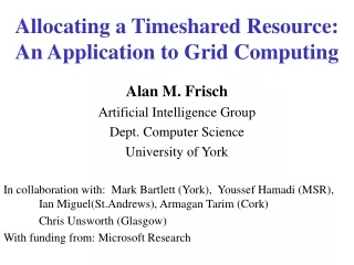
1. Allocating a Timeshared Resource:An Application to Grid Computing Alan M. Frisch Artificial Intelligence Group Dept. Computer Science University of York In collaboration with: Mark Bartlett (York), Youssef Hamadi (MSR), Ian Miguel(St.Andrews), Armagan Tarim (Cork) Chris Unsworth (Glasgow) With funding from: Microsoft Research

2. Introduction • Effective use of grid computing will require efficient methods to solve a variety of combinatorial problems, such as: • Resource allocation, • Configuration, and • Scheduling. • Grid resources are not currently reserved in advance, but will in future.

3. Advanced Reservation • This talk considers to the problem of allocating a time-shared or space-shared resource to bids for advanced reservations. • Communication bandwidth • Computer memory or disk space • Equivalent rooms in a hotel that handles block booking • Use combinatorial optimisation methods • Constraint programming • Operations research: optimisation • Artificial intelligence: search

4. Simple Model of Advanced Reservation • Given bids for quantities of the resource, each offering a price: • Accept a subset of the bids that can be fulfilled and maximises revenue. • This talk presents an algorithm for solving large instances of this problem in batch mode.

5. Temporal Knapsack Problem (TKP) • Given: • A finite set of times totally ordered by  • Along with each time t, capacity(t), a positive integer • A finite set of bids • Along with each bid b • price(b), demand(b), two positive integers • duration(b), a non-empty interval of times • Find: a set accept bids • Such that: t  times  demand(b)  capacity(t) b  accept|t  duration(b) • Maximising:price(b) b  accept

6. Solution: Objective Fn = £21 Bid1: 6 units, £11 Bid2: 6 units, £10 t1 t2 t3 t4 t5 Sample Instance of TKP Uniform Capacity: 10 Bid1: 6 units, £11 Bid2: 6 units, £10 Bid3: 5 units, £20 t1 t2 t3 t4 t5

7. TKP Generalises Knapsack • Every instance of Knapsack is an instance of TKP in which |times| = 1. • Hence TKP is NP-hard. (Easy to see that TKP is NP-easy)

8. Multi-dimensional Knapsack (MDK) generalises TKP • Multi-dimensional knapsack • each item has n-dimensional vector as its size • knapsack has n-dimensional vector as its capacity • sum of sizes of items in knapsack cannot exceed capacity of knapsack • Every instance of TKP is an instance of MDK in which the times are the dimensions and every item has size of form (0 … 0 demand … demand 0 … 0)

9. TKP Reduces toInteger Linear Programming Uniform Capacity: 10 Bid1: 6 units, £11 Bid2: 6 units, £10 Bid3: 5 units, £20 t1 t2 t3 t4 t5 Maximise: SXb price(b) b  bids 6X2  10 Subject to: b Xb in {0,1} 6X2+ 5X3  10 5X3  10 • 6X1 + 5X3  10 6X1  10

10. Solving the TKP • Decomposition algorithm • Greedy Algorithm (approximation) • Integer Linear Programming: CPLEX

11. Decomposition Algorithm

12. Decomposition Algorithm • Makes use of three operations: • Reduce the problem into a simpler one • Split into independent sub-problems. • Branch on accept/reject a bid. • These operations are composed into a branch and bound search for optimal solutions.

13. t1 t2 t3 t4 t5 t6 t7 t8 t9 Reduce: Forced Reject • If at any time during the interval required by a bid, available bandwidth is less than that requested, bid rejected. Bid: 10 units required. 10 AvailableCapacity: 5

14. t10 t12 t11 t5 t9 t6 t6 t7 t5 t2 t8 t1 t3 t4 t8 6 6 • Problem reduced to important decision points. 5 Reduce: Remove Times Bid1: 6 units Bid2: 6 units Bid3: 5 units Capacity: 10 Demand:

15. t10 t11 t12 t4 t4 t3 t9 t8 t2 t6 t6 t5 t5 t1 t7 6 • Bid1 Accepted. 5 Reduce: Remove Times  Forced Accept Bid1: 4 units Bid2: 6 units Bid3: 5 units Capacity: 10 Demand:

16. t10 t11 t12 t2 t1 t9 t8 t7 t6 t5 t3 t4 t6 Split Bid1: 6 units Bid2: 6 units Bid3: 5 units • Can solve independently, combine solutions. AND Bid1: 6 units Bid2: 6 units Bid3: 5 units t1 t2 t3 t4 t5 t6 t6 t7 t8 t9 t10 t11 t12

17. t5 t8 t5 t8 t8 t5 6 6 5 Branch Demand 11 Capacity 10 Accept Blue OR Reject Blue 6 6 6 6 Demand 6 Capacity 10 Capacity 5 Demand 6

18. t5 t6 t6 t7 t8 t9 t1 t2 t3 t4 Interaction: Example Bid1: 6 units • Bid 1: Forced reject. Bid2: 5 units Capacity: Demand:

19. t5 t6 t6 t7 t8 t9 t1 t2 t3 t4 Interaction: Example • Times removed. So bid 2 accepted. Bid2: 5 units Capacity: Demand:

20. Decomposition Algorithm: Initialisation(P) • Reduce(P) • Split P into set of problems S. • Foreach sS, Solve(s).

21. Decomposition Algorithm: Solve(P) • If no bids, return. • Select a bid b from bids. • Branch on: • Reject(b) then Reduce(P). Split(P) into set of problems S. Foreach sS, Solve(s). • Accept(b) then Reduce(P). Split(P) into set of problems S. Foreach sS, Solve(s).

22. Deterministic Algorithm:AND/OR Search Space A,B,C,D,E,F Reject A  Accept B Accept A  Reject C,D B,E,F C,D,E,F AND Split Split B,E,F E,F C,D

23. A Solution is a Tree A,B,C,D,E,F Reject A  Accept B Accept A  Reject C,D B,E,F AND Split Split B,E,F E,F C,D

24. Growing the AND/OR Tree • While tree contains an OR node with bids do • Choose one such OR node, N • Choose a bid in N; call it b • Generate two children of N by branching on b • Reduce each child • Split each child • How to choose node to expand, N • Or partially-grown solution tree • How to choose bid to branch on, b

25. Propagating Bounds [36 46] A,B,C,D,E,F Accept A (10) Reject C,D Reject A Accept B (11) B,E,F [15 35] C,D,E,F [25 35] AND Split Split B,E,F E,F C,D [15 35] [15 20] [10 15]

26. Using Bounds: Branch and Bound [46 61] A,B,C,D,E,F Accept A (10) Reject C,D Reject A Accept B (11) B,E,F [15 35] C,D,E,F [36 50] AND Split Split B,E,F E,F C,D [15 35] [15 20] [21 30]

27. Using Bounds: Branch and Bound [46 61] A,B,C,D,E,F Accept A (10) Reject C,D Reject A Accept B (11) B,E,F [15 35] C,D,E,F [36 50] AND Split Split B,E,F E,F C,D [15 35] [15 20] [21 30]

28. Choosing a Node: Search Strategy • AO* • Expand tree with highest upper bound • Admissible: first solution found is best • Optimal: expands fewest possible nodes for any given upper-bound method • Uses a lot of memory • Depth First • Expand deepest node • Uses little memory, but expands more nodes than AO*

29. Choosing a Bid to Branch on • Longest Duration: choose bid with longest duration • Intuition: maximise reduction; get the most information from one choice • Force splits: choose adjacent times and branch on all bids that span those two times. • Consequence: we can split problem between the two times. • Intuition: maximise splitting • Trade-off between splitting into equal subproblems and minimising number of branches. • In our experiments forced splits always outperformed longest duration.

30. Performance

31. Compare Performance of Three Solvers • Decomposition algorithm with depth-first search. • Decomposition algorithm with AO* search. • CPLEX on ILP formulation

32. Generating Random Instances • Given parameters: max-rate, number of bids • Allocate resources for a period of one month. Granularity of 15 minutes, gives 2,880 times. • Start time of each bid: uniform random [1, 2880] • Duration of each bid: uniform random [1, 100] • Bandwidth of each bid: uniform random [1, 50] • Rate of each bid: uniform random [1, max-rate] • Price and end time of each bid derived from above.

33. Experimental Results • Number of bids: 400, 450, 500, 550, 600 • MaxRate: 1.0, 1.2, 1.4, 1.6, 1.8, 2.0 • As MaxRate increases, the instances become harder for all solvers.

34. Experimental Results • Now consider performance as num of bids varies. • Use force-splits for decomposition algorithm • For each number of bids, used a suite of instances with 20 members from each max-rate value. • Up to 550 orders: all algorithms less than 10 secs. • Over 550, AO* runs out of memory. • Over 600, depth-first decomposition too slow. • Over 650, CPLEX runs out of memory.

35. Summary and Future Directions

36. Summary • Defined TKP and identified it as a model of advanced reservation • Presented special-purpose algorithm for TKP • Decomposition is distinctive feature

37. Future Directions: Improve Current Solver • Employ a search algorithm that takes middle ground between time-hungry, space-efficient DFS time-efficient, space-hungry AO* • adapt a space-bounded search algorithm to AND/OR • Better heuristic for choosing where to force splits Careful tradeoff between advantages of • minimising branching needed to force a split • splitting into equal-sized subproblems • Better data structures • Identify more redundant times

38. Future Directions: Improve Model of Advanced Reservation • Allow flexibility in time requested by a bid • Accommodate multiple resources and combined bids • Dynamic environment • Bids arrive as jobs are being executed • Some jobs can be thrown out or rescheduled, perhaps with a penalty • Some jobs may terminate early

39. Further Information www.cs.york.ac.uk/aig/constraints/Grid Frisch@cs.york.ac.uk