Download
1 / 21
210 likes | 215 Views
Spectral partitioning works: Planar graphs and finite element meshes. Daniel A. Spielman, Shang-Hua Teng Presented By Yariv Yaari. Paper Result. Spectral partitioning on a planar graph of bounded degree will find a cut of ratio

E N D
Spectral partitioning works: Planar graphs and finite element meshes Daniel A. Spielman, Shang-Hua Teng Presented By Yariv Yaari
Paper Result • Spectral partitioning on a planar graph of bounded degree will find a cut of ratio • Similar results for k-nearest neighbor graphs in a fixed dimension
Outline • Introduction • Spectral Partitioning • Bound on Fiedler value using Embedding • Bound for Planar graphs • Bisection from low-ratio cut • Questions?
Introduction • Our goal is to find good partitioning of graphs. (also called cut) • Partition of G=(V,E) is , we define • Good partition, large and small • The cut ratio is
The Laplacian • The Laplacian of a graph G, L(G) is an nxn matrix with entries defined by E. • For G=(V,E), , and • We are interested in eigenvalues, eigenvectors of the Laplacian.
Spectral Partitioning • Partition the graph using an eigenvector of the Laplacian. • Choose a number s and split v into: and • There are several approaches to choose s, we will only consider the choice optimizing the cut’s ratio, and only for an eigenvector of a specific eigenvalue, Fiedler value.
The Laplacian - properties • For any vector x, • Therefore, L(G) is symmetric positive semidefinite matrix, all eigenvalues are non-negative reals. • 0 is always an eigenvalue. If G is connected, its eigenvectors are spanned by (1,1,1,…,1). • The second smallest eigenvalue is called Fiedler value.
Fielder Value • Since L(G) is symmetric, the eigenvectors are orthogonal and we get • The minimized quotient is called Rayleigh Quotient, and it can be used to find a low ratio cut.
Rayleigh quotient • (Mihail): for a graph G of maximum degree d, for any vector x s.t. There is s such that the cut have ratio at most • Therefore, we want to bind Fiedler value.
Embedding • We will find a bound using an embedding into Rm. • We use: where • This is a direct result of the one-dimensional case.
“Kissing Disk” embedding • (Koebe–Andreev–Thurston): For any planar graph G=(V,E) there are disks with pair wise disjoint interiors s.t.
Sphere Preserving maps • A sphere preserving map is a map f s.t. the image of any sphere under f is a sphere and similarly the pre-image. • We will use sphere preserving maps between a sphere and a hyperplane. • For our purposes, a hyperplane is a sphere, so a möbius transformation is sphere preserving.
Bound for planar graphs • We will soon prove the existence of a sphere preserving map from the plane to the sphere s.t. the centroid of the centers of the disks is the origin. • Then denote the centers, the radii, we then get and for all i,j Therefore we can split it between i and j and get the bound But the caps are disjoint, so
Bound for planar graphs - cont. • Also, • So, summing everything we get • Therefore, and using its eigenvector one can find a cut of ratio
Sphere preserving maps - cont • We want a sphere preserving map that will map centers of spheres to a set on a sphere with the centroid at the origin. • First, build a family of sphere preserving maps. • For a sphere and a point denote the stereographic projection of the sphere on the extended hyperplane tangent to the sphere at (extended, with infinity point). This is sphere preserving.
Sphere preserving maps - cont • Any möbius transformation is sphere preserving, we will only use dilation, denote a dilation with factor around by • Any composition of Sphere preserving maps is sphere preserving • Our family of sphere preserving functions will be
Sphere preserving maps - cont • We now extend the definition for as (this is not continuous) • Now, for a cap C on the unit sphere denote its center by we would like to show that for all there is s.t.
Sphere preserving maps - cont • We will need that there is no point shared by the interior of at least half of the caps (in current case, the interiors are disjoint). • We would like to use a mapping from to the centroid of however, this map is not continuous. • Choose s.t. for all , most of the caps are contained within a ball of radius around
Sphere preserving maps - cont • Now define a weight function: • And so
Sphere preserving maps - cont • is continuous and approach zero where is not continuous, so is continuous. • Now, if the centers are in or and most of them in . Therefore lies on line between the origin and • This implies (by Brewer’s fixed point), and we’re done.