Download
1 / 101
1.15k likes | 2.42k Views
Finite Element Modeling and Analysis. CE 595: Course Part 2 Amit H. Varma. Discussion of planar elements. Constant Strain Triangle (CST) - easiest and simplest finite element Displacement field in terms of generalized coordinates Resulting strain field is

E N D
Finite Element Modeling and Analysis CE 595: Course Part 2 Amit H. Varma
Discussion of planar elements • Constant Strain Triangle (CST) - easiest and simplest finite element • Displacement field in terms of generalized coordinates • Resulting strain field is • Strains do not vary within the element. Hence, the name constant strain triangle (CST) • Other elements are not so lucky. • Can also be called linear triangle because displacement field is linear in x and y - sides remain straight.
Constant Strain Triangle • The strain field from the shape functions looks like: • Where, xi and yi are nodal coordinates (i=1, 2, 3) • xij = xi - xj and yij=yi - yj • 2A is twice the area of the triangle, 2A = x21y31-x31y21 • Node numbering is arbitrary except that the sequence 123 must go clockwise around the element if A is to be positive.
Constant Strain Triangle • Stiffness matrix for element k =BTEB tA • The CST gives good results in regions of the FE model where there is little strain gradient • Otherwise it does not work well. If you use CST to model bending. See the stress along the x-axis - it should be zero. The predictions of deflection and stress are poor Spurious shear stress when bent Mesh refinement will help.
Linear Strain Triangle • Changes the shape functions and results in quadratic displacement distributions and linear strain distributions within the element.
Linear Strain Triangle • Will this element work better for the problem?
Example Problem • Consider the problem we were looking at: 1k 1 in. 1k 5 in. 0.1 in.
Bilinear Quadratic • The Q4 element is a quadrilateral element that has four nodes. In terms of generalized coordinates, its displacement field is:
Bilinear Quadratic • Shape functions and strain-displacement matrix
Bilinear Quadratic • The element stiffness matrix is obtained the same way • A big challenge with this element is that the displacement field has a bilinear approximation, which means that the strains vary linearly in the two directions. But, the linear variation does not change along the length of the element. y, v y x, u y x varies with y but not with x y varies with x but not with y x x x y
Bilinear Quadratic • So, this element will struggle to model the behavior of a beam with moment varying along the length. • Inspite of the fact that it has linearly varying strains - it will struggle to model when M varies along the length. • Another big challenge with this element is that the displacement functions force the edges to remain straight - no curving during deformation.
Bilinear Quadratic • The sides of the element remain straight - as a result the angle between the sides changes. • Even for the case of pure bending, the element will develop a change in angle between the sides - which corresponds to the development of a spurious shear stress. • The Q4 element will resist even pure bending by developing both normal and shear stresses. This makes it too stiff in bending. • The element converges properly with mesh refinement and in most problems works better than the CST element.
Example Problem • Consider the problem we were looking at: 0.1k 1 in. 0.1k 5 in. 0.1 in.
Quadratic Quadrilateral Element • The 8 noded quadratic quadrilateral element uses quadratic functions for the displacements
Quadratic Quadrilateral Element • Shape function examples: • Strain distribution within the element
Quadratic Quadrilateral Element • Should we try to use this element to solve our problem? • Or try fixing the Q4 element for our purposes. • Hmm… tough choice.
y 4 3 M1 M2 b x 1 2 a Improved Bilinear Quadratic (Q6) • The principal defect of the Q4 element is its overstiffness in bending. • For the situation shown below, you can use the strain displacement relations, stress-strain relations, and stress resultant equation to determine the relationship between M1 and M2 • M2 increases infinitely as the element aspect ratio (a/b) becomes larger. This phenomenon is known as locking. • It is recommended to not use the Q4 element with too large aspect ratios - as it will have infinite stiffness
Improved bilinear quadratic (Q6) • One approach is to fix the problem by making a simple modification, which results in an element referred sometimes as a Q6 element • Its displacement functions for u and v contain six shape functions instead of four. • The displacement field is augmented by modes that describe the state of constant curvature. • Consider the modes associated with degrees of freedom g2 and g3.
Improved Bilinear Quadratic • These corrections allow the elements to curve between the nodes and model bending with x or y axis as the neutral axis. • In pure bending the shear stress in the element will be • The negative terms balance out the positive terms. • The error in the shear strain is minimized.
Improved Bilinear Quadratic • The additional degrees of freedom g1 - g4 are condensed out before the element stiffness matrix is developed. Static condensation is one of the ways. • The element can model pure bending exactly, if it is rectangular in shape. • This element has become very popular and in many softwares, they don’t even tell you that the Q4 element is actually a modified (or tweaked) Q4 element that will work better. • Important to note that g1-g4 are internal degrees of freedom and unlike nodal d.o.f. they are not connected to to other elements. • Modes associated with d.o.f. gi are incompatible or non-conforming.
Improved bilinear quadratic • Under some loading, on overlap or gap may be present between elements • Not all but some loading conditions this will happen. • This is different from the original Q4 element and is a violation of physical continuum laws. • Then why is it acceptable? Elements approach a state Of cons
No numbers! What happened here?
Discontinuity! Discontinuity! Discontinuity!
Q6 or Q4 with incompatible modes Why is it stepped? Note the discontinuities LST elements Q4 elements Q8 elements Why is it stepped? Small discontinuities?
Q6 or Q4 with incompatible modes LST elements Q4 elements Q8 elements
Q6 or Q4 with incompatible modes LST elements Discontinuities Accurate shear stress? Q4 elements Q8 elements Some issues!
Lets refine the Q8 model. Quadruple the number of elements - replace 1 by 4 (keeping the same aspect ratio but finer mesh). Fix the boundary conditions to include additional nodes as shown Define boundary on the edge! Black Black Black The contours look great! So, why is it over-predicting?? The principal stresses look great Is there a problem here?
Shear stresses look good But, what is going on at the support Why is there S22 at the supports? Is my model wrong?
Reading assignment • Section 3.8 • Figure 3.10-2 and associated text • Mechanical loads consist of concentrated loads at nodes, surface tractions, and body forces. • Traction and body forces cannot be applied directly to the FE model. Nodal loads can be applied. • They must be converted to equivalent nodal loads. Consider the case of plane stress with translational d.o.f at the nodes. • A surface traction can act on boundaries of the FE mesh. Of course, it can also be applied to the interior.
Equivalent Nodal Loads • Traction has arbitrary orientation with respect to the boundary but is usually expressed in terms of the components normal and tangent to the boundary.
Principal of equivalent work • The boundary tractions (and body forces) acting on the element sides are converted into equivalent nodal loads. • The work done by the nodal loads going through the nodal displacements is equal to the work done by the the tractions (or body forces) undergoing the side displacements
Body Forces • Body force (weight) converted to equivalent nodal loads. Interesting results for LST and Q8
Important Limitation • These elements have displacement degrees of freedom only. So what is wrong with the picture below? Is this the way to fix it?
Stress Analysis y • Stress tensor • If you consider two coordinate systems (xyz) and (XYZ) with the same origin • The cosines of the angles between the coordinate axes (x,y,z) and the axes (X, Y, Z) are as follows • Each entry is the cosine of the angle between the coordinate axes designated at the top of the column and to the left of the row. (Example, l1=cos xX, l2=cos xY) Y z x z X
Stress Analysis • The direction cosines follow the equations: • For the row elements: li2+mi2+ni2=1 for I=1..3 l1l2+m1m2+n1n2=0 l1l3+m1m3+n1n3=0 l3l2+m3m2+n3n2=0 • For the column elements: l12+l22+l32=1 Similarly, sum (mi2)=1 and sum(ni2)=1 l1m1+l2m2+l3m3=0 l1n1+l2n2+l3n3=0 n1m1+n2m2+n3m3=0 • The stresses in the coordinates XYZ will be:
Stress Analysis • Principal stresses are the normal stresses on the principal planes where the shear stresses become zero • P=N where is the magnitude and N is unit normal to the principal plane • Let N = l i + m j +n k (direction cosines) • Projections of P along x, y, z axes are Px= l, Py= m, Pz= n Equations A
Stress Analysis • Force equilibrium requires that: l (xx-) + m xy +n xz=0 l xy + m (yy-) + n yz = 0 l xz + m yz + n (zz-) = 0 • Therefore, Equations B Equation C
Stress Analysis • The three roots of the equation are the principal stresses (3). The three terms I1, I2, and I3 are stress invariants. • That means, any xyz direction, the stress components will be different but I1, I2, and I3 will be the same. • Why? --- Hmm…. • In terms of principal stresses, the stress invariants are: I1= p1+p2+p3 ; I2=p1p2+p2p3+p1p3 ; I3 = p1p2p3 • In case you were wondering, the directions of the principal stresses are calculated by substituting =p1 and calculating the corresponding l, m, n using Equations (B).
Stress Analysis • The stress tensor can be discretized into two parts: = + Original element Volume change Distortion only - no volume change m is referred as the mean stress, or hydostatic pressure, or just pressure (PRESS)
Stress Analysis • In terms of principal stresses
Stress Analysis • The Von-mises stress is • The Tresca stress is max {(p1-p2), (p1-p3), (p2-p3)} • Why did we obtain this? Why is this important? And what does it mean? • Hmmm….
Isoparametric Elements and Solution • Biggest breakthrough in the implementation of the finite element method is the development of an isoparametric element with capabilities to model structure (problem) geometries of any shape and size. • The whole idea works on mapping. • The element in the real structure is mapped to an ‘imaginary’ element in an ideal coordinate system • The solution to the stress analysis problem is easy and known for the ‘imaginary’ element • These solutions are mapped back to the element in the real structure. • All the loads and boundary conditions are also mapped from the real to the ‘imaginary’ element in this approach
Y,v X, u Isoparametric Element 3 4 (x3, y3) 4 3 (x4, y4) (1, 1) (-1, 1) 2 1 (-1, -1) (1, -1) 2 1 (x2, y2) (x1, y1)
Isoparametric element • The mapping functions are quite simple: Basically, the x and y coordinates of any point in the element are interpolations of the nodal (corner) coordinates. From the Q4 element, the bilinear shape functions are borrowed to be used as the interpolation functions. They readily satisfy the boundary values too.
Isoparametric element • Nodal shape functions for displacements
Isoparametric Element Hence we will do it another way
Isoparametric Element The remaining strains y and xy are computed similarly The element stiffness matrix dX dY=|J| dd
Gauss Quadrature • The mapping approach requires us to be able to evaluate the integrations within the domain (-1…1) of the functions shown. • Integration can be done analytically by using closed-form formulas from a table of integrals (Nah..) • Or numerical integration can be performed • Gauss quadrature is the more common form of numerical integration - better suited for numerical analysis and finite element method. • It evaluated the integral of a function as a sum of a finite number of terms