Download
1 / 24
240 likes | 313 Views
Optimized Yield Curve Matching. Mark Davenport 3 December 2007. Outline. Motivation Financial Background Black Box Optimizer Alternative Objective Functions Simulations Results Conclusion. Motivation. Employee pension benefits provide flows of income to retired or disable employees

E N D
Optimized Yield Curve Matching Mark Davenport 3 December 2007
Outline • Motivation • Financial Background • Black Box Optimizer • Alternative Objective Functions • Simulations • Results • Conclusion
Motivation • Employee pension benefits provide flows of income to retired or disable employees • Pension funds provide the necessary cash flows to cover these pension obligations • The goal of managing these funds is to ensure sufficient cash flows • The focus of this project will be how to best manage the risks associated with attaining this goal
Financial Background • Price-yield relationship of a bond • Shifts in the yield curve cause PV of bond to change • Duration • Measure of sensitivity of the price of a bond to changes in interest rate • Portfolio Immunization • Practice of minimizing amount of interest rate risk to a portfolio • This project explores a duration matching strategy
Black Box Optimizer • Optimization routine using Excel Solver • Allocates plan across grouping of assets • Initial point • Random proportion of plan size assigned to each bond • Total amount allocated equals plan size • Test of assumption • 6 Yield Curves, 3 random starting points • Average difference between points • $28,969 – trivial considering over $1 billion plan size
Optimization Routine C: difference in contribution to duration T: total plan size B: amount invested D: duration w: maximum relative $ duration v, u: minimum amount invested
Alternative Objective Functions • Twofold Process • Five objective function structures • Four weighting strategies • Total of 20 objective functions tested • Benchmark Objective Function • NISA’s Current Strategy • Subtle implicit weighting • Questionable: • Not enough emphasis on short term • Single year diluted across entire investment horizon
Weighting Schemes • Implicit Weighting • Apply weight = 1 for each observation • Simple Short-Term Weighting • Apply weight = 1- • Power Weighting • Apply power of six to first ten years, power of four to the next twenty years, power of two for the remaining • Simple Weight-to-End • Apply weight =
Simulation • As input, used single upward sloping yield curve • Created portfolio for each objective function
Volatility • Three volatility environments • Moderate • Extreme • NISA
Moderate Volatility • Two shift scenarios • Short-Term & Long-Term • For each, 3 types of shifts • 100 basis point shift • 200 basis point shift • 50 basis point bend
Extreme Volatility • Examined Short-Term, Long-Term, and Constant volatility scenarios
NISA Volatility • Generated in-house at NISA • Assuming to be closest proxy for true Yield Curve volatility • Used as benchmark for my volatility
Determining Results • Results based off of 50,000 simulated yield curve shifts observed for each objective function • Difference in PV of assets and liabilities recorded • Standard deviation of differences determined the tracking error for each environment • Reported as raw number and in % of liability
Results – Objective Functions • Best for Short-Term Volatility in all environments • Least Squares Method • Two-Period Lagged Method (only power-weighted and simple weight-to-end strategies) • Best for Constant and Long-Term Extreme Volatility • Five Period Lagged Method • Change in Summation Method
Results – Weighting Strategies • No impact on Least Squares Method • Short-Term Weighting Strategy in general • Encouraging results for power weighted benchmark and two-period lagged methods • In general, best for extreme short-term and extreme constant volatility
Results – Weighting Strategies • Long-Term Weighting • Not a well designed test because cash flows resulting past 40 year mark are essentially zero • However, still positive results • Simple weight-to-end best for moderate long-term volatility, also for moderate short-term volatility • Oddly, generated better results as compared to short-term weighting strategy
Discussion • Least Squares and Two-Period Lagged (power weighted and simple weight-to-end) Methods
Discussion • Five-Period Lagged and Change in Summation Methods
Discussion – Which is “best”? • Different yield curve environments require different objectives • Similarly, different money managing styles require different objectives • Reallocate once a day? Month? Decade? • “Best” objective? • Moderate short term volatility most realistic • Least Squares or Two-Period Lagged
Extensions • Interface Excel and Matlab • Take advantage of strength of Matlab’s NLP capability • Introduce knowledge of convexity of assets and liability • Explore stronger short term weighting strategies • Introduce more asset classes into the problem • Become more interesting • Eliminate skewing effect of large 30 year cash flow • Explore different inputs
Accomplishments • Optimizer can identify global minimum • Simulated results determined better optimization routine • Given the constraints of the problem • Demonstrated importance of design in solving this problem • Knowledge of external factors