Download
1 / 75
790 likes | 1.14k Views
Growth Curve Models. Thanks due to Betsy McCoach David A. Kenny August 26, 2011. Overview. Introduction Estimation of the Basic Model Nonlinear Effects Exogenous Variables Multivariate Growth Models. Not Discussed or Briefly Discussed (see extra slides at the end).

E N D
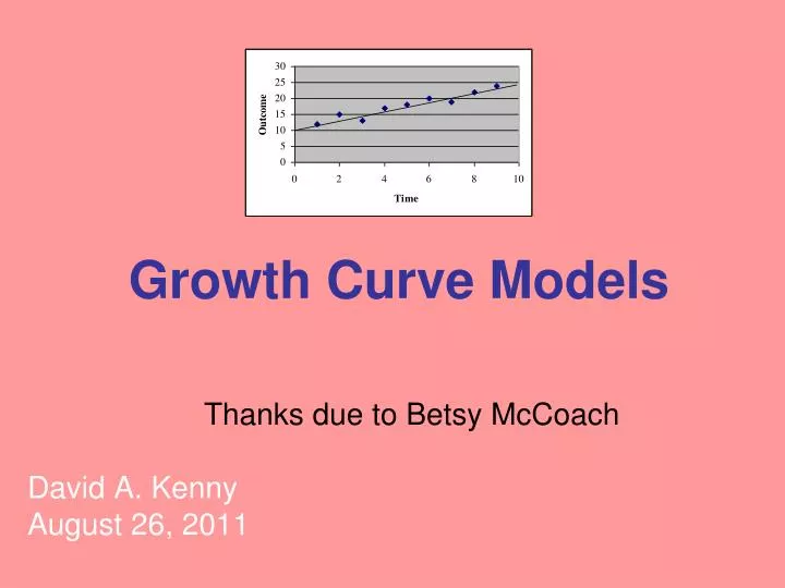
Growth Curve Models Thanks due to Betsy McCoach David A. Kenny August 26, 2011
Overview • Introduction • Estimation of the Basic Model • Nonlinear Effects • Exogenous Variables • Multivariate Growth Models
Not Discussed or Briefly Discussed (see extra slides at the end) • Modeling Nonlinearity • LDS Model • Time-varying Covariates • Point of Minimal Intercept Variance • Complex Nonlinear Models
Two Basic Change Models • Stochastic • I am like how I was, but I change randomly. • These random “shocks” are incorporated into who I am. • Autoregressive models • Growth Curve Models • Each of us in a definite track. • We may be knocked off that track, but eventually we end up “back on track.” • Individuals are on different tracks.
Linear Growth Curve Models • We have at least three time points for each individual. • We fit a straight line for each person: • The parameters from these lines describe the person.
The Key Parameters • Slope: the rate of change • Some people are changing more than others and so have larger slopes. • Some people are improving or growing (positive slopes). • Some are declining (negative slopes). • Some are not changing (zero slopes). • Intercept: where the person starts • Error: How far the score is from the line.
Latent Growth Models (LGM) • For both the slope and intercept there is a mean and a variance. • Mean • Intercept: Where does the average person start? • Slope: What is the average rate of change? • Variance • Intercept: How much do individuals differ in where they start? • Slope: How much do individuals differ in their rates of change: “Different slopes for different folks.”
Measurement Over Time • measures taken over time • chronological time: 2006, 2007, 2008 • personal time: 5 years old, 6, and 7 • missing data not problematic • person fails to show up at age 6 • unequal spacing of observations not problematic • measures at 2000, 2001, 2002, and 2006
Data • Types • Raw data • Covariance matrix plus means Means become knowns: T(T + 3)/2 Should not use CFI and TLI (unless the independence model is recomputed; zero correlations, free variances, means equal) • Program reproduces variances, covariances (correlations), and means.
Independence Model • Default model in Amos is wrong! • No correlations, free variances, and equal means. • df of T(T + 1)/2 – 1
Specification: Two Latent Variables • Latent intercept factor and latent slope factor • Slope and intercept factors are correlated. • Error variances are estimated with a zero intercept. • Intercept factor • free mean and variance • all measures have loadings set to one
Slope Factor • free mean and variance • loadings define the meaning of time • Standard specification (given equal spacing) • time 1 is given a loading of 0 • time 2 a loading of 1 • and so on • A one unit difference defines the unit of time. So if days are measured, we could have time be in days (0 for day 1 and 1 for day 2), weeks (1/7 for day 2), months (1/30) or years (1/365).
Time Zero • Where the slope has a zero loading defines time zero. • At time zero, the intercept is defined. • Rescaling of time: • 0 loading at time 1 ─ centered at initial status • standard approach • 0 loading at the last wave ─ centered at final status • useful in intervention studies • 0 loading in the middle wave ─ centered in the middle of data collection • intercept like the mean of observations
Different Choices Result In • Same • model fit (c2 or RMSEA) • slope mean and variance • error variances • Different • mean and variance for the intercept • slope-intercept covariance
some intercept variance, and slope and intercept being positively correlated no intercept variance intercept variance, with slope and intercept being negatively correlated
Identification • Need at least three waves (T = 3) • Need more waves for more complicated models • Knowns = number of variances, covariances, and means or T(T + 3)/2 • So for 4 times there are 4 variances, 6 covariances, and 4 means = 14 • Unknowns • 2 variances, one for slope and one for intercept • 2 means, one for the slope and one for the intercept • T error variances • 1 slope-intercept covariance
Model df • Known minus unknowns • General formula: T(T + 3)/2 – T – 5 • Specific applications • If T = 3, df = 9 – 8 = 1 • If T = 4, df = 14 – 9 = 5 • If T = 5, df = 20 – 10 = 10
Three-wave Model • Has one df. • The over-identifying restriction is: M1 + M3 – 2M2 = 0 (where “M” is mean) i.e., the means have a linear relationship with respect to time.
Example Data • Curran, P. J. (2000) • Adolescents, ages 10.5 to 15.5 at Time 1 • 3 times, separated by a year • N = 363 • Measure • Perceived peer alcohol use • 0 to 7 scale, composite of 4 items
Parameter Estimates Estimate SE CR MEANS Intercept 1.304 .091 14.395 Slope 0.555 .050 11.155 VARIANCES Intercept 2.424 .300 8.074 Slope 0.403 .132 3.051 Error1 0.596 .244 2.441 Error2 1.236 .143 8.670 Error3 1.492 .291 5.132 COVARIANCE* Intercept-Slope -0.374 .163 -2.297 *Correlation = -.378
Interpretation • Mean • Intercept: The average person starts at 1.304. • Slope: The average rate of change per year is .555 units. • Variance • Intercept • +1 sd = 1.30 + 1.56 = 2.86 • -1 sd = 1.30 – 1.56 = -0.26 • Slope • +1 sd = .56 + .63 =1.19 • -1 sd = .56 – .63 = -0.07 • % positive slopes P(Z > -.555/.634) = .80
Model Fit c2(1) = 4.98, p = .026 RMSEA = .105 CFI = (442.49 – 5 – 4.98 + 1)/ (442.49 – 5) = .991 Conclusion: Good fitting model. (Note that the RMSEA with small df can be misleading.)
NonlinearityLatent Basis Model: Some Loadings Free • Fix the loadings for two waves of data to different nonzero values and free the other loadings. In essence rescales time.
Results for Alcohol Data Wave 1: 0.00 Wave 2: 0.84 Wave 3: 2.00 Function fairly linear as 0.84 is close to 1.00.
Trimming Growth Curve Models • Almost never trim • Slope-intercept covariance • Intercept variance • Never have the intercept “cause” the slope factor or vice versa. • Slope variance: OK to trim, i.e., set to zero. • If trimmed set slope-intercept covariance to zero. • Do not interpret standardized estimates except the slope-intercept correlation.
Using Amos • Must tell the Amos to “Estimate means and intercepts.” • Growth curve plug-in • It names parameters, sets measures’ intercepts to zero, frees slope and intercept factors’ means and variance, sets error variance equal over time, fixes intercept loadings to 1, and fixes slope loadings from 0 to 1.
Second Example • Ormel, J., & Schaufeli, W. B. (1991). Stability and change in psychological distress and their relationship with self-esteem and locus of control: A dynamic equilibrium model. Journal of Personality and Social Psychology, 60, 288-299. • 389 Dutch Adults after College Graduation • 5 Waves Every Six Months • Distress Measure
Parameter Estimates Estimate SE CR MEANS Intercept 3.276 .156 20.946 Slope -0.043 .040 -1.079 VARIANCES Intercept 6.558 .707 9.272 Slope 0.170 .052 3.250 All error variances statistically significant COVARIANCE* Intercept-Slope -0.458 .156 -2.926 *Correlation = -.433
Interpretation Large variance in distress level. Average slope is essentially zero. Variance in slope so some are increasing in distress and others are declining. Those beginning at high levels of distress decline over time.
Model Fit c2(10) = 110.37, p < .001 RMSEA = .161 CFI = (895.35 – 14 – 110.35 + 10)/ (895.35 – 14) = .886 Conclusion: Poor fitting model.
Alternative Options for Error Variances • Force error variances to be equal across time. • c2(4) = 19.1 (not helpful) • Non-independent errors • errors of adjacent waves correlated • c2(4) = 10.4 (not much help) • autoregressive errors (err1 err2 err3) • c2(4) = 10.5 (not much help)
Exogenous Variables • Often in this context referred to as “covariates” • Types • Person – e.g., age and gender • Time varying: a different measure at each time • See “extra” slides. • Need to center (i.e., remove their mean) these variables. • For time-varying use one common mean.
Person Covariates • Center (failing the center makes average slope and intercept difficult to interpret) • These variables explain variation in slope and intercept; have an R2. • Have them cause slope and intercept factors. • Intercept: If you score higher on the covariate, do you start ahead or behind (assuming time 1 is time zero)? • Slope: If you score higher on the covariate, do you grow at a faster and slower rate. • Slope and intercept now have intercepts not means. Their disturbances are correlated.
Three exogenous person variables predict the slope and the intercept (own drinking)
Effects of Exogenous Variables Variable Intercept Slope Age .606* .057 Gender -.113 .527* COA .462 .705* R2 .101 .054 c2(4) = 4.9 Intercept: Older children start out higher. Slope: More change for Boys and Children of Alcoholics. (Trimming ok here.)
Extra Slides • Relationship to multilevel models • Time varying covariates • Multivariate growth curve model • Point of minimal intercept variance • Other ways of modeling nonlinearity • Empirically scaling the effect of time • Latent difference scores • Non-linear dynamic models
Relationship to Multilevel Modeling (MLM) • Equivalent if ML option is chosen • Advantages of SEM • Measures of absolute fit • Easier to respecify; more options for respecification • More flexibility in the error covariance structure • Easier to specify changes in slope loadings over time • Allows latent covariates • Allows missing data in covariates • Advantages of MLM • Better with time-unstructured data • Easier with many times • Better with fewer participants • Easier with time-varying covariates • Random effects of time-varying covariates allowable
Time-Varying Covariates • A covariate for each time point. • Center using time 1 mean (or the mean at time zero.) • Do not have the variable cause slope or intercept. • Main Effect • Have each cause its measurement at its time. • Set equal to get the main effect. • Interaction: Allow the covariate to have a different effect at each time.
Interpretation • Main effects of the covariate. • Path: .504 (p < .001) • c2(3) = 8.44, RMSEA = .071 • Peer “affects” own drinking • Covariate by Time interaction • Chi square difference test: c2(2) = 4.24, p = .109 • No strong evidence that the effect of peer changes over time.
Results • Main effects model • Interaction model • Changes the intercept at each time. • Covariate acts like a step function.
Covariate by Time Interaction • Covariate by Time (linear), Phantom variable approach
Partner Drinking as a Time-varying Covariate: V1 and V2 Are Latent Variables with No Disturbance (Phantom Variables)
Results • Main Effect of Peer: 0.376 (p = .038) • Time x Peer: 0.107 (p = .427) • The effect of Peer increases over time, but not significantly.