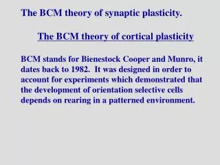
Download
1 / 62
710 likes | 1.08k Views
The BCM theory of synaptic plasticity. c. m. 1. m. 3. m. 2. d. d. d. 1. 2. 3. Output. Simple Model of a Neuron. Synaptic weights. Inputs. c. æ. ö. n. å. =. s. ×. ç. ÷. c. m. d. i. i. è. ø. =. 1. i. (. ). =. s. ×. m. d. m. ». ×. m. d. 1. m. 3. m.

E N D
c m 1 m 3 m 2 d d d 1 2 3 Output Simple Model of a Neuron Synaptic weights Inputs
c æ ö n å = s × ç ÷ c m d i i è ø = 1 i ( ) = s × m d m » × m d 1 m 3 m 2 ( ) s × m d × m d d d d 1 2 3 Output Neuron Activation Synaptic weights Inputs
c c » × c m d m m m d d d Output signal Output increase Output decrease Synaptic Modification Synaptic weight Weight increase Weight decrease Input signal
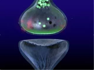
dm = i cd i dt Hebbian Learning “When an axon in cell A is near enough to excite cell B and repeatedly and persistently takes part in firing it, some growth process or metabolic change takes place in one or both cells such that A’s efficiency in firing B is increased.” - Hebb, 1949 “Those that fire together wire together” • Mathematically:
dm = i cd i dt dm = i cd i environmen t dt environmen t å = m d d j j i j environmen t å = m d d j j i environmen t j å = C m ij j j Stability and Behavior of Hebbian Learning • Unstable as written: requires synaptic decrease • Finds correlations in environment
dm d m å = = i C m Cm ij j dt dt j dm da å = a i v a dt dt a å å = = l a Cv a v a a a a a a a da l = = l t a a ( t ) a ( 0 ) e a a a a a a dt Hebbian Learning and Principal Components • Matrix equivalent of Hebbian Learning • Eigenvectors of C, the principle components: • Expand in terms of eigenvectors, : • Component with largest eigenvalue wins
Mathematical method implies Biological mechanism Synaptic Stabilization • Saturation limits • Normalization • Decay terms • Moving threshold Synaptic weights (Linsker 1986;Miller 1994) (Oja 1982, Blais et. al. 1998) (BCM 1982, IC 1992; Blais et. al. 1999)
Combining Hebbian and Anti-Hebbian Learning • A more general Hebbian-like rule • Includes a decrease of weights in • For response increases • For response decreases • Yields selectivity… • … but not stable
BCM Theory (Bienenstock, Cooper, Munro 1982; Intrator, Cooper 1992) • Selectivity learning rule with moving threshold • Time average of the square of the neuron activity
dm = h f q j d ( c , ) j M dt [ ] q µ = 2 E c M t 1 ò ¢ ¢ ¢ - - t 2 ( t t ) / c ( t ) e d t t -¥ (Bienenstock, Cooper, Munro 1982; Intrator, Cooper 1992) BCM Theory Requires • Bidirectional synaptic modification LTP/LTD • Sliding modification threshold • The fixed points depend on the environment, and in a patterned environment only selective fixed points are stable. LTD LTP
t 1 ò ¢ ¢ ¢ - - t q = 2 ( ) / t t c ( t ) e d t M t - ¥ q d 1 = - q 2 m ( c ) m t dt The integral form of the average: Is equivalent to this differential form:
BCM TheoryStability • One dimension • Quadratic form • Instantaneous limit
æ ö æ ö 1 . 0 0 . 1 ç ÷ ç ÷ = = 1 2 d d ç ÷ ç ÷ 0 . 2 0 . 9 è ø è ø What is the outcome of the BCM theory? Assume a neuron with N inputs (N synapses), and an environment composed of N different input vectors. A N=2 example: What are the stable fixed points of m in this case?
= × i i c m d (Notation: ) Note:Every time a new input is presented, m changes, and so does θm What are the fixed points? What are the stable fixed points?
Two examples with N= 5 Note: The stable FP is such that for one pattern ci=mdi=θm while for the othersC(i≠j)=0.
BCM TheoryStability • One dimension • Quadratic form • Instantaneous limit
BCM TheorySelectivity • Two dimensions • Two patterns • Quadratic form • Averaged threshold , • Fixed points
BCM Theory: Selectivity • Learning Equation • Four possible fixed points , (unselective) , (Selective) , (Selective) , (unselective) • Threshold
BCM Theory: Stability • Learning Equation • Four possible fixed points , (unstable) , (stable) , (stable) , (unstable) only selective fixed points are stable • Threshold
Ex1 - Final Task • Create a BCM learning rule which can go into the Fast ICA algorithm of Hyvarinen. • Run it on multi modal distributions as well as other distributions. • Running should be as the regular fast ICA but with a new option for the BCM rule. • Demonstrate how down in Fisher score can you go to still get separation
Left Right Tuning curves Response (spikes/sec) 0 90 180 270 360 Right Left
LTD 1 5 0 1 2 5 % of baseline 1 0 0 7 5 1 H z 5 0 - 3 0 - 1 5 0 1 5 3 0 4 5 T i m e f r o m o n s e t o f L F S ( m i n ) LTP 2 0 0 % of baseline 1 5 0 1 0 0 HFS 5 0 - 1 5 0 1 5 3 0 Time (min) Ocular Dominance Plasticity (Mioche and Singer, 89) Synaptic plasticity in Visual Cortex (Kirkwood and Bear, 94 ) Receptive field Plasticity Left Eye Right Eye R e c o r d S t i m u l a t e
light electrical signals Visual Cortex Receptive fields are: • Binocular • Orientation Selective Visual Pathway Area 17 LGN Receptive fields are: • Monocular • Radially Symmetric Retina
Image plane Right Retina Left Retina LGN LGN Right Synapses Left Synapses Cortex (single cell) Model Architecture Inputs Synaptic weights Output
Binocular Deprivation Normal Orientation Selectivity Adult Response (spikes/sec) Response (spikes/sec) Adult angle angle Eye-opening Eye-opening
20 30 % of cells 15 10 1 2 3 4 5 6 7 Monocular Deprivation Normal Left Right Right Left Response (spikes/sec) angle angle 1 2 3 4 5 6 7 Rittenhouseet. al. group group
retinal activity image Natural Images, Noise, and Learning • present patches • update weights • Patches from retinal activity image • Patches from noise
(Mioche, Singer 1989) 20 N=33 15 Number of cells 10 5 0 Both Left Right • Synaptic weights output properties Cortical Properties and Synapses • Orientation selectivity • responds to bars of light at a particular orientation • elongated regions of strong synapses • Binocularity • responds to both eyes • similar synapse configuration from each eye
Orientation selectivity • responds to bars of light at a particular orientation • elongated regions of strong synapses Hebbian Learning and Orientation Selectivity experiment simulation
Orientation selectivity • responds to bars of light at a particular orientation • elongated regions of strong synapses BCM Learning and Orientation Selectivity experiment simulation
Left Right Hebbian Learning Right Eye Left Right Left Eye Binocularity BCM Learning Right Synapses Left Synapses
PCA Right Eye Left Eye Left Right 100 50 0 100 Right Synapses 50 Left Synapses 0 No. of Cells 100 50 0 100 50 0 1 2 3 Bin Orientation selectivity and Ocular Dominance
100 50 0 100 50 0 No. of Cells 40 20 0 100 50 0 1 2 3 4 5 Bin Right Eye BCM neurons can develop both orientation selectivity and varying degrees of Ocular Dominance Left Eye Right Synapses Left Synapses Shouval et. al., Neural Computation, 1996
(Mioche, Singer 1989) 20 N=33 15 Number of cells 10 5 0 Both Right Left N=42 Selectivity 0 1 2 3 4 5 6 Days • Monocular deprivation (MD) • in 12 hours, responds more strongly to open eye • synapses from closed eye weaken • Binocular deprivation (BD) • in 3-4 days, responses are smaller from both eyes • all synapses are weakened, but more slowly than MD Cortical Properties and Synapses (adapted from Freeman et. Al. 1981)
Observation • Loss of response during Monocular Deprivation is much more rapid than during Binocular Deprivation. (Hubel and Wiesel, 1963, 1965) • Therefore the two eyes compete for limited resources. • Mechanism: Synaptic competition.
Normalization implies competition • for weights to increase, others decrease • Monocular deprivation (MD) • open eye weights are driven up • closed eye weights are driven down • more activity in closed eye reduces driving force • No competition in binocular deprivation Synaptic Competition and Monocular Deprivation open eye response closed eye time (Mioche, Singer 1989) 20 N=33 15 Number of cells 10 5 0 Both Right Left
A stabilized Hebb rule: Oja rule (PCA) If Many variants: Stent (73), von der Malsburg (73), Miller (89) ... | || | || | | | || | | | | | { Heterosynaptic LTD
open eye response closed eye time q M f ( c ) f » - e ( 0 ) c 2 f q » + e - q ( ) ( c ) M 1 M • Temporal competition between incoming patterns • For a selective neuron, most responses are… BCM Theory and Monocular Deprivation • ~ 0 for non-optimum patterns • ~ for optimum patterns • Linear approximation of
Pattern into open eye, • Noise into closed eye, • Output depends on pattern and noise • Two cases of patterns into the open eye • non-optimum patterns BCM Theory and Monocular Deprivation • optimum patterns
Two cases of patterns into the open eye • non-optimum patterns • optimum patterns BCM Theory and Monocular Deprivation • For a selective neuron, • closed eye weights decrease • more activity in the closed eye increases the effect
Right Both Left weak activity strong activity • Synaptic competition • more activity into closed eye decreases shift in responses toward open eye • BCM Theory • more activity into closed eye increases shift in responses toward open eye Summary of Theory Number of cells Right Both Left Number of cells Right Both Left Left Right Both
weak activity 160 160 N=238 N=273 120 120 Number of cells 80 80 40 40 0 0 Right Both Left Right Both Left Number of cells Right Both Left Right Both Left Number of cells Right Both Left Left Right Both strong activity • Rittenhouse et. al. 1999 • TTX in retina • consistent with BCM Experiment and Theory • Synaptic competition • BCM Theory
Monocular DeprivationHomosynaptic model (BCM) Low noise High noise
Monocular DeprivationHeterosynaptic model (K2) Low noise High noise