Download
1 / 49
490 likes | 516 Views
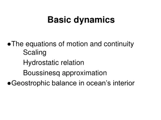
Basic dynamics ●The equations of motion and continuity Scaling Hydrostatic relation Boussinesq approximation ●Geostrophic balance in ocean’s interior. The Equation of Motion. Newton’s second law in a rotating frame. (Navier-Stokes equation).

E N D
Basic dynamics ●The equations of motion and continuity Scaling Hydrostatic relation Boussinesq approximation ●Geostrophic balance in ocean’s interior
The Equation of Motion Newton’s second law in a rotating frame.(Navier-Stokes equation) : Acceleration relative to axis fixed to the earth. : Pressure gradient force. : Coriolis force, where : Effective (apparent) gravity. : Friction. molecular kinematic viscosity.
Gravity: Equal Potential Surfaces • g changes about 5% 9.78m/s2 at the equator (centrifugal acceleration 0.034m/s2, radius 22 km longer) 9.83m/s2 at the poles) • equal potential surface normal to the gravitational vector constant potential energy the largest departure of the mean sea surface from the “level” surface is about 2m (slope 10-5) • The mean ocean surface is not flat and smooth earth is not homogeneous
Given the zonal momentum equation If we assume the turbulent perturbation of density is small i.e., The mean zonal momentum equation is Where Fx is the turbulent (eddy) dissipation If the turbulent flow is incompressible, i.e.,
Eddy Dissipation Reynolds stress tensor and eddy viscosity: , Then Where the turbulent viscosity coefficients are anisotropic. Ax=Ay~102-105 m2/s Az ~10-4-10-2 m2/s >>
Reynolds stress has no symmetry: A more general definition: if (incompressible)
Continuity Equation Mass conservation law In Cartesian coordinates, we have or For incompressible fluid, If we define and , the equation becomes
Scaling of the equation of motion • Consider mid-latitude (φ≈45o) open ocean away from strong current and below sea surface. The basic scales and constants: L=1000 km = 106 m H=103 m U= 0.1 m/s T=106 s (~ 10 days) 2Ωsin45o=2Ωcos45o≈2x7.3x10-5x0.71=10-4s-1 g≈10 m/s2 ρ≈103 kg/m3 Ax=Ay=105 m2/s Az=10-1 m2/s • Derived scale from the continuity equation W=UH/L=10-4 m/s
Scaling the vertical component of the equation of motion Hydrostatic Equation accuracy 1 part in 106
Boussinesq approximation Density variations can be neglected for its effect on mass but not on weight (or buoyancy). where , we have Assume that where Then the equations are (1) (2) where (3) (The term (4) is neglected in (1) for energy consideration.)
Scaling of the horizontal components (accuracy, 1% ~ 1‰) Zero order (Geostrophic) balance Pressure gradient force = Coriolis force
Re-scaling the vertical momentum equation Since the density and pressure perturbation is not negligible in the vertical momentum equation, i.e., , and , The vertical pressure gradient force becomes
Taking into the vertical momentum equation, we have , and assume If we scale then and (accuracy ~ 1‰)
Geopotential Geopotential Φis defined as the amount of work done to move a parcel of unit mass through a vertical distance dz against gravity is The geopotential difference between levels z1 and z2 (with pressure p1 and p2) is (unit of Φ: Joules/kg=m2/s2).
Dynamic height , we have Given where is standard geopotential distance (function of p only) is geopotential anomaly. In general, Φ is sometime measured by the unit “dynamic meter” (1dyn m = 10 J/kg). which is also called as “dynamic height” (D) Units: δ~m3/kg, p~Pa, D~ dyn m Note: Though named as a distance, dynamic height (D) is still a measure of energy per unit mass.
Geopotential and isobaric surfaces Geopotential surface: constant Φ, perpendicular to gravitiy, also referred to as “level surface” Isobaric surface: constant p. The pressure gradient force is perpendicular to the isobaric surface. In a “stationary” state (u=v=w=0), isobaric surfaces must be level (parallel to geopotential surfaces). In general, an isobaric surface (dashed line in the figure) is inclined to the level surface (full line). In a “steady” state ( ), the vertical balance of forces is The horizontal component of the pressure gradient force is
Geostrophic relation The horizontal balance of force is where tan(i) is the slope of the isobaric surface. tan (i) ≈ 10-5 (1m/100km) if V1=1 m/s at 45oN (Gulf Stream). • In principle, V1 can be determined by tan(i). In practice, tan(i) is hard to measure because • p should be determined with the necessary accuracy • (2) the slope of sea surface (of magnitude <10-5) can not be directly measured (probably except for recent altimetry measurements from satellite.) (Sea surface is a isobaric surface but is not usually a leveled surface.)
Calculating geostrophic velocity using hydrographic data The difference between the slopes (i1 and i2) at two levels (z1 and z1) can be determined from vertical profiles of density observations. Level 1: Level 2: Difference: i.e., because A1C1=A2C2=L and B1C1-B2C2=B1B2-C1C2 because C1C2=A1A2 Note that z is negative below sea surface.
Since , and we have The geostrophic equation becomes
“Thermal Wind” Equation Starting from geostrophic relation Differentiating with respect to z Using Boussinesq approximation Or Rule of thumb: light water on the right. .
, The geostrophic current we calculate is actually the “Thermal Wind” Analytically, or similarly
Since currents in deep ocean are much weak, there may exist a level (z2) where v1 >> v2 so that we can reasonably assume v2≈0 (level of no motion (LNM)). Then The rule for direction is the same for both p and ΔD. In practice, however, we see sections of hydrographic data (T, S, or σt). In that case, A rule for current direction is: (In northern hemisphere) Relative to the water below it, the current flows with the “lighter water on its right” In a vertical section, the isopycnals (curves of constant ρ or δ) slope downward from left to right. With respect to temperature, it is the “warmer water on its right”
Level of No Motion (LNM) Pacific: Deep water is uniform, current is weak below 1000m. Atlantic: A level of no motion at 1000-2000m “Slope current”: Relative geostrophic current is zero but absolute current is not. May occurs in deep ocean (barotropic?) Current increases into the deep ocean, unlikely in the real ocean
Barotropic flow: p and ρ surfaces are parallel For a barotropic flow, we have is geostrophic current. Since Given a barotropic and hydrostatic conditions, and Therefore, And So (≈0 in Boussinesq approximation)
Baroclinic Flow: and There is no simple relation between the isobars and isopycnals. slope of isobar is proportional to velocity slope of isopycnal is proportional to vertical wind shear.
1½ layer flow Simplest case of baroclinic flow: Two layer flow of density ρ1 and ρ2. The sea surface height is η=η(x,y) (In steady state, η=0). The depth of the upper layer is at z=d(x,y). The lower layer is at rest. For z > d, For z ≤ d, If we assume The slope of the interface between the two layers (isopycnal)= times the slope of the surface (isobar). The isopycnal slope is opposite in sign to the isobaric slope.
σt A B diff 26.8 50m --- >50m 27.0 130m 280m -150m 27.7 579m 750m -180m Isopycnals are nearly flat at 100m Isobars ascend about 0.13m between A and B for upper 150m Below 100m, isopycnals and isobars slope in opposite directions with 1000 times in size.
Summary • In practice, geostrophic method yields only relative currents and the selection of an appropriate level of no motion always presents a problem. • One is faced with a problem when the selected level of no motion reaches the ocean bottom as the stations get close to shore. • It only yields mean values between stations which are many tens of kilometers apart. • Friction has been ignored. • The balance breaks down near the equator (within ±0.5o latitude (i.e., ±50km) of the equator).
Properties of Sea Water • What is the pressure at the bottom of the ocean relative to sea surface pressure? What unit of pressure is very similar to 1 meter? • What is salinity and why do we use a single chemical constituent (which one?) to determine it? What other physical property of seawater is used to determine salinity? What are the problems with both of these methods? • What properties of seawater determine its density? What is an equation of state? • What happens to the temperature of a parcel of water (or any fluid or gas) when it is compressed adiabatically? What quantity describes the effect of compression on temperature? How does this quantity differ from the measured temperature? (Is it larger or smaller at depth?) • What are the two effects of adiabatic compression on density? • What are σt and σθ? How do they different from the in situ density? • Why do we use different reference pressure levels for potential density? • What are the significant differences between freezing pure water and freezing seawater?
Basic Dynamics • What are the differences between the centrifugal force and the Coriolis force? Why do we treat them differently in the primitive equation? • What is the definition of dynamic height? • In geostrophic flow, what direction is the Coriolis force in relation to the pressure gradient force? What direction is it in relation to the velocity? • Why do we use a method to get current based on temperature and salinity instead of direct current measurements for most of the ocean? • How are temperature and salinity information used to calculate currents? What are the drawbacks to this method? • What is a "level of no motion"? Why do we need a "level of known motion" for the calculation of the geostrophic current? (What can we actually compute about the velocity structure given the density distribution and an assumption of geostrophy?) • What are the barotropic and baroclinic flows? Is there a “thermal wind” in a barotropic flow? • What can you expect about the relation between the slopes of the thermocline depth and the sea surface height?