Download
1 / 35
450 likes | 967 Views
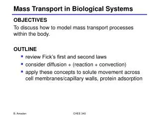
MEDE 3005 Transport Phenomena for Biological Systems. Dr. K. W. Chow (3 weeks) – Basic principles of fluid dynamics; Conservation laws of mass and momentum; Continuity of equations; Euler’s and Navier Stokes equations of motion. Dr. C. O. Ng (3 weeks) Dr. L. Q. Wang (the rest of the course).

E N D
MEDE 3005Transport Phenomena for Biological Systems Dr. K. W. Chow (3 weeks) – Basic principles of fluid dynamics; Conservation laws of mass and momentum; Continuity of equations; Euler’s and Navier Stokes equations of motion. Dr. C. O. Ng (3 weeks) Dr. L. Q. Wang (the rest of the course)
Basic Concepts in Fluid Flows Dependence of time and space (a) Steady uniform flows – properties independent of time and space; (b) Steady non-uniform flows – properties independent of time but depend on space (e.g. converging channels) (c) Unsteady uniform flows – properties depending on time but not on space (e.g. turning on a faucet slowly) (d) Unsteady non-uniform flows – properties depending on space and time.
Real and ideal fluids:(1) Ideal fluid – no friction, fluid can ‘slide’ tangentially along the solid boundary.(2) Real fluid – will possess friction (or viscosity), fluid cannot ‘slide’ along boundary – no slip boundary condition.Tangential velocity = zero if the wall is at rest.(3) Velocity component perpendicular to the wall must be the same as that of the wall – no penetration condition (= zero if the wall is at rest).
(1) Incompressible flows – density of the fluid remains constant. Otherwise compressible fluid.(Strictly speaking: incompressible flow refers to the material derivative of the density being zero)In practice, compressible if the Mach number about 0.5 or so.Sound speed = 340 m per s.(2) 1D, 2D, 3D (dimensional) flows
(1) Differential (versus integral or macroscopic, i.e. control surfaces, control volume types) Analysis of Fluid Motions (2) Conservation of mass, momentum and energy. Incompressible fluids – no need to use the energy equation. (3) Material derivative = Derivative following the particle as it flows
Eulerian versus Lagrangian descriptionsof fluid motion Eulerian – fixed coordinates, do not follow particles, velocity expressed as functions of spatial coordinates, i.e. different particles will flow through the same point at different times. Most fluid mechanics textbooks and papers use this system, i.e. more common than the Lagrangian method.
Eulerian versus Lagrangian descriptionsof fluid motion (cont’d) Lagrangian – follow individual particles, positions of specified particles are the objectives. Can employ the more familiar Newton’s laws of motion but less convenient for applications. Main difficulty is that we have billions of fluid particles and not just one or two.
Vorticity = curl of the velocity field= twice the local angular velocity of the fluid
Differential analysis of the motion of a fluid element(1) Translation,(2) Angular distortion,(3) Rotation (related to the vorticity),(4) Volume distortion (zero if the fluid is of constant density).
Continuity Equation – Conservation of Mass Mass outflux = mass influx + flow due to source(s) – flow due to sink(s) Volume flux = velocity X (area) = velocity X (length) X depth normal to page Mass flux = density X (volume flux)
Incompressible flows (constant density)Derivation of the continuity equation in Cartesian coordinates.
Incompressible flows (constant density)Continuity equation = divergence of the velocity field = 0.
Continuity equation(1) in three dimensions;(2) in polar coordinates;(3) in summation convention.
Reynolds number = (reference velocity) X (reference length)/(kinematic viscosity)Shear stress = (Dynamic viscosity) X (velocity gradient)Kinematic viscosity = (Dynamic viscosity)/density
Reynolds number = (inertial force)/(viscous force)Inertial force = Mass X AccelerationRe >> 1, viscosity not important;Re << 1, viscous effects dominant.What is driving the fluid motion?
Laminar flow – slow, regular motion.Turbulent flow – fast, chaotic motion.Transition – from laminar to turbulent flows.
Inviscid Equations of Motion= Euler’s equation of motion Mass X (acceleration) = Mass X (MATERIAL DERIVATIVE of the velocity field) = Force = (usually due to force from the pressure gradient alone) (Exceptions : additional body force due stratification, rotation, electric charge etc)
Acceleration in terms of the Eulerian descriptionacceleration = (velocity at t + dt – velocity at t)/dt as dt tends to zero,but velocity = a function of (t, x, y, z) in the Eulerian description. For 2 D flows, by using a Taylor’s expansion (say x direction):∂u/∂t + (∂u/∂x)(dx/dt) + (∂u/∂y)(dy/dt)= ∂u/∂t + u(∂u/∂x) + v(∂u/∂y)
Stream functionDefinition of streamlines:A line (or more precisely a curve) such that the tangent to the curve is PARALLEL to the velocity vector.As such the flow or the particles will move along the streamlines.
Mathematicallyu = ∂Ψ/∂y v = – ∂Ψ/∂xas follows from a consideration of Ψ = constant and take the differential dΨ = 0. Analytically, the stream function is a mathematical device to satisfy the continuity equation identically (note that ux + vy = 0 automatically)
The Navier Stokes equations – equations of motion for a viscous fluid (Note : the principle of conservation of mass, or continuity equation, holds whetherthe fluid is viscous or not. Eulerian description : Force = mass (acceleration) = mass (MATERIAL DERIVATIVE of the velocity) = net forces
Viscous versus Ideal Fluids : (1) For a viscous fluid (a fluid with friction), there will be tangential as well as normal stresses. (2) Net Forces = Small differences due to differential changes in stresses (similar to the treatment in solid mechanics).
Relation(s) between stress and strain = Constitutive equations.(Analytical details in notes)In terms of (usual) symbols(i) Solid mechanics – u, v, w displacements(ii) Fluid mechanics – u, v, w velocities
Non-dimensionalizing the equations of motion:Convective acceleration terms;Pressure gradient terms;Body force terms;New ingredients: VISCOUS terms
Boundary Conditions(1) Ideal Fluid – no penetration, or the normal velocitiesmust match. However, the fluid can still slide along the wall, i.e. the tangential velocities of the fluid and the wall need not match.
(2) Viscous Fluid – no penetration boundary condition, PLUS NO SLIP condition – fluid canNOT slide along the wall.
Flow of a viscous fluid along an inclined plane – gravity acts as the body force, and NO pressure gradient x, y axes along and normal to the inclined plane u = U(y), v = 0 No shear stress at free surface No slip at the wall
Flow along a horizontal, RECTANGULAR channel: No body force, and therefore must apply a pressure gradient. Otherwise the analysis is the same – u = U(y), v = 0, p = p(x) NO free surface, and hence no conditions involving the shear stress, instead, just no slip conditions at both walls.
Flow along a CIRCULAR pipe under constant pressure gradient No body force, and therefore we must apply a pressure gradient. The analysis and reasoning are the same as those in the rectangular channel case, but we must use polar coordinates.
Circular Pipe (cont’d) No radial nor tangential velocities. Only the axial velocity is nonzero: The continuity equation implies that the axial velocity does not depend on the axial coordinate. Equations of motion in the r and Θ directions imply that the pressure depends on the axial coordinate only.
Usual separation of variables approach to find the velocity profile as a function of radius and pressure gradient (which must be constant). Boundary conditions – no slip conditions at the wall, and the velocity must be finite at the center. (Two no slip conditions for fluids in an annular region).
Flow of a viscous fluid between co–rotating or counter–rotating cylinders: NO radial velocity; NO axial velocity; Only ‘tangential velocity’.
Continuity equation implies that this tangential velocity can only be a function of the radius. Can also be deduced from the axisymmetric requirement. Boundary conditions – ‘No slip’ will imply that the fluid will have an ‘angular velocity’ at the walls of the moving cylinder(s).
Coutte flow of a layered fluid Consider a 2-layer fluid between two rigid walls and NO pressure gradient is present. Motion is then driven by forcing one (or two) rigid wall(s) into motion. Equations of motion will continue to hold for both fluids, but we must also insist on some matching conditions at the interface.
Layered fluid (cont’d) Equations of motion will imply the second derivative of the velocity must be zero, and hence the velocity profile must be ‘piecewise linear’. No slip boundary conditions at both walls. At the interface, the velocity and the shear stress must be continuous. (Note: if the viscosities are different, => velocity gradients NOT continuous.)