Download
1 / 32
320 likes | 443 Views
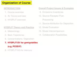
Organization of Course. Overall Project Issues & Examples Emissions Inventories Source-Receptor Post-Processing Source-Attribution for Deposition Model Evaluation Model Intercomparison Collaboration Possibilities. INTRODUCTION Course overview Air Toxics overview HYSPLIT overview

E N D
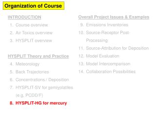
Organization of Course Overall Project Issues & Examples Emissions Inventories Source-Receptor Post-Processing Source-Attribution for Deposition Model Evaluation Model Intercomparison Collaboration Possibilities INTRODUCTION Course overview Air Toxics overview HYSPLIT overview HYSPLIT Theory and Practice Meteorology Back Trajectories Concentrations / Deposition HYSPLIT-SV for semivolatiles (e.g, PCDD/F) HYSPLIT-HG for mercury
Public Health Context • Methyl-mercury is a developmental neurotoxin -- risks to fetuses/infants • Cardiovascular toxicity might be even more significant (CRS, 2005) • Critical exposure pathway: methylmercury from fish consumption • Widespread fish consumption advisories • Uncertainties, but mercury toxicity relatively well understood • well-documented tragedies: (a) Minimata (Japan) ~1930 to ~1970; (b) Basra (Iraq), 1971 • epidemiological studies, e.g., (a) Seychelles; (b) Faroe Islands; (c) New Zealand • methylmercury vs. Omega-III Fatty Acids • selenium – protective role? • At current exposures, risk to large numbers of fetuses/infants + Wildlife Health Issues e.g., fish-eating birds
Different “forms” of mercury in the atmosphere • Elemental Mercury -- Hg(0) • most of total Hg in atmosphere • not very water soluble • doesn’t easily dry or wet deposit • upward evasion vs. deposition • atmos. lifetime approx ~ 0.5-1 yr • globally distributed Atmospheric methyl-mercury? • Reactive Gaseous Mercury -- RGM • a few percent of total atmos Hg • oxidized Hg (HgCl2, others) • operationally defined • very water soluble and “sticky” • atmos. lifetime <= 1 week • local and regional effects • bioavailable • Particulate Mercury -- Hg(p) • a few percent of total atmos Hg • not pure particles of mercury • Hg compounds in/on atmos particles • species largely unknown (HgO?) • atmos. lifetime approx 1~ 2 weeks • local and regional effects • bioavailability?
Hg from other sources: local, regional & more distant Reactive halogens in marine boundary layer emissions of Hg(0), Hg(II), Hg(p) • Enhanced oxidation of Hg(0) to RGM • Enhanced deposition wet and dry deposition to the watershed wet and dry deposition to the water surface Source Attribution for Deposition?
Elemental Mercury [Hg(0)] Upper atmospheric halogen-mediated oxidation? Polar sunrise “mercury depletion events” Hg(II), ionic mercury, RGM Particulate Mercury [Hg(p)] Br cloud CLOUD DROPLET Hg(II) reducedto Hg(0) by SO2 and sunlight Vapor phase: Hg(0) oxidized to RGM and Hg(p) by O3, H202, Cl2, OH, HCl Adsorption/ desorption of Hg(II) to /from soot Hg(p) Primary Anthropogenic Emissions Hg(0) oxidized to dissolved Hg(II) species by O3, OH, HOCl, OCl- Wet deposition Multi-media interface Dry deposition Re-emission of previously deposited anthropogenic and natural mercury Natural emissions Atmospheric Mercury Fate Processes
(Evolving) Atmospheric Chemical Reaction Scheme for Mercury ? ? new ?
Lagrangian Puff Atmospheric Fate and Transport Model 0 1 2 TIME (hours) The puff’s mass, size, and location are continuously tracked… = mass of pollutant (changes due to chemical transformations and deposition that occur at each time step) Phase partitioning and chemical transformations of pollutants within the puff are estimated at each time step Initial puff location is at source, with mass depending on emissions rate Centerline of puff motion determined by wind direction and velocity Dry and wet deposition of the pollutants in the puff are estimated at each time step. deposition 2 deposition to receptor deposition 1 lake NOAA HYSPLIT MODEL 8
Why are emissions speciation data - and potential plume transformations -- critical? Logarithmic NOTE: distance results averaged over all directions – Some directions will have higher fluxes, some will have lower
Why is emissions speciation information critical? Logarithmic Linear 12
The fraction deposited and the deposition flux are both important, but they have very different meanings… The fraction deposited nearby can be relatively “small”, But the area is also small, and the relative deposition flux can be very large… Cumulative Fraction Deposited Out to Different Distance Ranges from a Hypothetical Source 13
source location 0.1o x 0.1o subgrid for near-field analysis 14
deposition (ug/m2)* one Hg monitoring site 100 - 1000 10 – 100 1 - 10 0.1 – 1 Annapolis Washington D.C. Model-predicted hourly mercury deposition (wet + dry) in the vicinity of one example Hg source for a 3-day period in July 2007 one Hg emissions source * hourly deposition converted to annual equivalent
deposition (ug/m2)* one Hg monitoring site 100 - 1000 10 – 100 1 - 10 0.1 – 1 Annapolis Washington D.C. Model-predicted hourly mercury deposition (wet + dry) in the vicinity of one example Hg source for a 3-day period in July 2007 one Hg emissions source * hourly deposition converted to annual equivalent
Large, time-varying spatial gradients in deposition & source-receptor relationships deposition (ug/m2)* one Hg monitoring site 100 - 1000 10 – 100 1 - 10 0.1 – 1 Annapolis Washington D.C. Model-predicted hourly mercury deposition (wet + dry) in the vicinity of one example Hg source for a 3-day period in July 2007 one Hg emissions source * hourly deposition converted to annual equivalent
Exercise 8: • open up command prompt • navigate to c:\hysplit4\working_08 • cd c:\hysplit4\working_08 [enter] • run conc_run_08.bat • conc_run_08 [enter] Note – conc_run_08.bat CALLS conc_set_08.bat conc_set_08.bat is very complex If there is time, we can examine this batch file
Imported into Excel During the simulation, 1 gram/ hr was emitted, over 672 hours… A total of 672 grams of RGM were emitted The fraction of these emissions deposited in Lake Chapala was 0.17 / 672 = 0.00025 = 0.025% A total of 9% of the emissions were deposited during the simulation: 60 / 672 = 0.09 = 9%
Mercury Deposition (grams/day) to Lake Chapala arising from emissions of 1 gram/hr of Reactive Gaseous Mercury (RGM) from a source 40 km Northwest of the Lake Half of the total deposition to the Lake occurred in one day! Deposition (grams/day) Day of August 2008
In order to estimate the actual impact of a source, we multiply this unit-emissions result by the actual emissions For example, if the actual source emitted 1000 grams per day of RGM, then this simulation would imply that for Aug 2008, the source would contribute: 0.17 grams deposited per gram emitted * 1000 grams emitted = 170 grams to Lake Chapala
We have tried to extend the mercury modeling to a global basis, but have encountered problems
When puffs grow to sizes large relative to the meteorological data grid, they split, horizontally and/or vertically Ok for regional simulations, but for global modeling, puff splitting overwhelms computational resources
Due to puff splitting, the number of puffs quickly overwhelms numerical resources In this example, the maximum number of puffs was set to 100,000, so when it got close to that number, the splitting was turned off Exponential puff growth
In each test, the number of puffs rises to the maximum allowable within ~ one week This line is the example from the last slide
In the new version of HYSPLIT (4.9), puffs are “dumped” into an Eulerian grid after a specified time (e.g., 96 hrs), and the mercury is simulated on that grid from then on…
The version of HYSPLIT that we are running in this workshop has the Global Eulerian Model (GEM) integrated with the puff/particle model And a new version of the HYSPLIT-Hg model now includes this GEM integration We could run HYSPLIT-Hg / GEM at this workshop, but, it takes a little too long…